In today’s tutorial we investigate how you can use ThetaData’s API to retreive historical options data for end-of-day, and both intraday trades and quotes. We will create volatility surfaces use an interpolation method (B-Splines) to compare surfaces between the morning (10am) implied volalitity and afternoon (2pm) implied volatility surfaces.
import os
import time
import pickle
import numpy as np
import pandas as pd
import concurrent.futures as cf
import matplotlib.pyplot as plt

from datetime import timedelta, datetime, date
from thetadata import ThetaClient, OptionReqType, OptionRight, DateRange, DataType
To use the ThetaData API you will have to sign up for an account. Then you will pass your username and password as strings within the ThetaClient class init params.
Get all Expirations for SPY Options
your_username = ''
your_password = ''

def get_expirations(root_ticker) -> pd.DataFrame:
    """Request expirations from a particular options root"""
    # Create a ThetaClient
    client = ThetaClient(username=your_username, passwd=your_password, timeout=15)

    # Connect to the Terminal
    with client.connect():

        # Make the request
        data = client.get_expirations(
            root=root_ticker,
        )

    return data

root_ticker = 'SPY'
expirations = get_expirations(root_ticker)

root_ticker = 'SPY'
expirations = get_expirations(root_ticker)

exp_dates = expirations[expirations > time_now + timedelta(days=7)]
exp_dates
Get all Strikes for each SPY Option
def get_strikes(root_ticker, expiration_date) -> pd.DataFrame:
    """Request strikes from a particular option contract"""
    # Create a ThetaClient
    client = ThetaClient(username=your_username, passwd=your_password, timeout=15)

    # Connect to the Terminal
    with client.connect():

        # Make the request
        data = client.get_strikes(
            root=root_ticker,
            exp=expiration_date
        )

    return data

root_ticker = 'SPY'
exp_date = date(2022,9,16)
strikes = get_strikes(root_ticker, exp_date)
strikes

root_ticker = 'SPY'
all_strikes = {}
for exp_date in exp_dates:
    all_strikes[exp_date] = pd.to_numeric(get_strikes(root_ticker, exp_date))
Find combined Strikes across expiry dates
Using set intersection of all strikes across SPY Options contracts.
Save strikes down with pickle for use later.
combined_strikes = [list(strikes) for strikes in all_strikes.values()]
vol_surface_strikes = set.intersection(*map(set,combined_strikes))
vol_surface_strikes

with open('vol_surface_strikes.pkl', 'wb') as f:
    pickle.dump(vol_surface_strikes, f)

with open('vol_surface_strikes.pkl', 'rb') as f:
    vol_surface_strikes = pickle.load(f)

vol_surface_strikes = list(vol_surface_strikes)
vol_surface_strikes.sort()
vol_surface_strikes
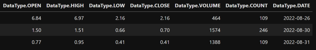
Retreive EOD Options Data
def end_of_day(root_ticker, exp_date, strike, from_date, to_date) -> pd.DataFrame:
    """Request end-of-day data"""
    # Create a ThetaClient
    client = ThetaClient(username=your_username, passwd=your_password, timeout=10)

    # Connect to the Terminal
    with client.connect():

        # Make the request
        data = client.get_hist_option(
            req=OptionReqType.EOD,
            root=root_ticker,
            exp=exp_date,
            strike=strike,
            right=OptionRight.CALL,
            date_range=DateRange(from_date, to_date),
        )

    return data

root_ticker = 'SPY'
from_date = date(2022,8,26)
to_date = date(2022,8,31)
exp_date = exp_dates.tolist()[0]
strike = 420000
data = end_of_day(root_ticker, exp_date, int(int(strike)/1000), from_date, to_date)
data
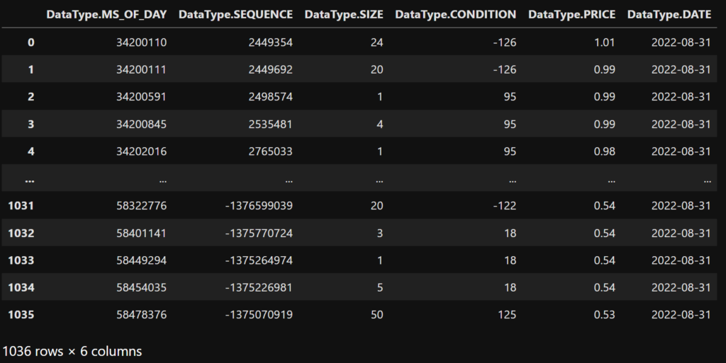
Retreive Trades Data
# Make the request
def trades(root_ticker, exp_date, strike, from_date, to_date) -> pd.DataFrame:
    """Request trade level data"""
    # Create a ThetaClient
    client = ThetaClient(username=your_username, passwd=your_password, timeout=10)

    # Connect to the Terminal
    with client.connect():

        data = client.get_hist_option(
            req=OptionReqType.TRADE,
            root=root_ticker,
            exp=exp_date,
            strike=strike,
            right=OptionRight.CALL,
            date_range=DateRange(from_date, to_date),
            progress_bar=False,
        )

    return data


root_ticker = 'SPY'
exp_date = date(2022,9,16)
from_date = date(2022,8,31)
to_date = date(2022,8,31)
strike = 420000
data = trades(root_ticker, exp_date, int(int(strike)/1000), from_date, to_date)
data
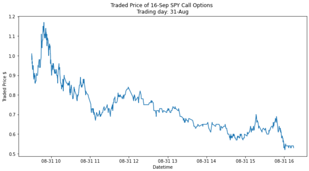
Use MS_OF_DAY to Create DateTime
data['DATETIME'] = data[DataType.DATE] + pd.TimedeltaIndex(data[DataType.MS_OF_DAY], unit='ms')
plt.figure(figsize=(12,6))
plt.title('Traded Price of 16-Sep SPY Call Options \n Trading day: 31-Aug ')
plt.xlabel('Datetime')
plt.ylabel('Traded Price $')
plt.plot(data['DATETIME'],data[DataType.PRICE])
Retreive Quoted Intraday Options Prices
# Make the request
def quotes(root_ticker, exp_date, strike, from_date, to_date, interval_size=0) -> pd.DataFrame:
    """Request quotes both bid/ask options data"""
    # Create a ThetaClient
    client = ThetaClient(username=your_username, passwd=your_password, timeout=10)

    # Connect to the Terminal
    with client.connect():

        data = client.get_hist_option(
            req=OptionReqType.QUOTE,
            root=root_ticker,
            exp=exp_date,
            strike=strike,
            right=OptionRight.CALL,
            date_range=DateRange(from_date, to_date),
            progress_bar=False,
            interval_size=interval_size
        )

    return data


root_ticker = 'SPY'
exp_date = date(2022,9,16)
from_date = date(2022,8,31)
to_date = date(2022,8,31)
strike = 420000
data = quotes(root_ticker, exp_date, int(int(strike)/1000), from_date, to_date)
data
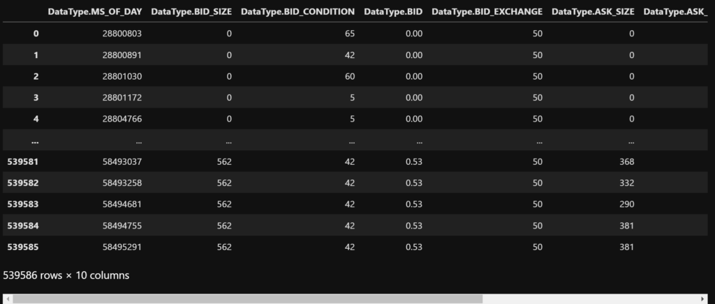
Change interval size
Aggregate average BID/ASK Quotes on a 5 minute basis.
interval_size = 5*60000
data = quotes(root_ticker, exp_date, int(int(strike)/1000), from_date, to_date, interval_size)
dt_date_ms = data[DataType.DATE] + pd.TimedeltaIndex(data[DataType.MS_OF_DAY], unit='ms')
data.insert(loc=0, column='DATETIME', value=dt_date_ms)
data

morning_int = 120
afternoon_int = 168
morning = data['DATETIME'][morning_int]
afternoon = data['DATETIME'][afternoon_int]
print("Morning Interval", morning, "\nAfternoon Interval", afternoon)

data.iloc[afternoon_int]
Calculate Weighted Mid Price (Micro-Price)
Calculate the weighted mid price (micro-price) for each row within our quotes dataframe.
$$\Large P_{m} = P_a \frac{V_b}{(V_a + V_b)} + P_b \frac{V_a}{(V_a + V_b)}$$
def weighted_mid_price(row):
    try:
        V_mid = row[DataType.ASK_SIZE] + row[DataType.BID_SIZE]
        x_a = row[DataType.ASK_SIZE]/V_mid
        x_b = 1 - x_a
        return row[DataType.ASK]*x_a + row[DataType.BID]*x_b
    except:
        return np.nan

midprices = data.apply(weighted_mid_price, axis=1)
midprices
Create request for 10:00 and 14:00 Weighted Mid Prices
# Make the request
def get_morn_noon_quotes(root_ticker, exp_date, strike, from_date, to_date, interval_size=0) -> pd.DataFrame:
    """Returns morning and afternoon weighter mid prices at 1000 and 1400 respectively"""
    # Create a ThetaClient
    client = ThetaClient(username=your_username, passwd=your_password, timeout=10)

    # Connect to the Terminal
    with client.connect():

        data = client.get_hist_option(
            req=OptionReqType.QUOTE,
            root=root_ticker,
            exp=exp_date,
            strike=strike,
            right=OptionRight.CALL,
            date_range=DateRange(from_date, to_date),
            progress_bar=False,
            interval_size=interval_size
        )

    morning_int = 120
    afternoon_int = 168

    midprices = data.apply(weighted_mid_price, axis=1)

    return midprices[morning_int], midprices[afternoon_int]
Multi-threading Responses to ThetaData API
Now we explore using current.futures module to perform multi-threading and processing of responses using ThetaData API.
- We need to create a function that we can call with our specific parameters of interest
- We need to know the maximium number of threads our computer has
def retrieve_eod_data(root_ticker, exp_date, strike, from_date, to_date, interval_size):
    try:
        morning, afternoon = get_morn_noon_quotes(root_ticker, exp_date, int(int(strike)/1000), from_date, to_date, interval_size)
        print("  ", strike," data")
        datas[exp_date][strike] = [morning, afternoon]
    except:
        datas[exp_date][strike] = [np.nan, np.nan]
        print("  ", strike," no data")


root_ticker = 'SPY'
from_date = date(2022,8,31)
to_date = date(2022,8,31)
interval_size = 5*60000

datas = {}
for exp_date in exp_dates:
    print(exp_date)
    start = time.time()
    datas[exp_date] = {}
    executor = cf.ThreadPoolExecutor(8)
    futures = [executor.submit(retrieve_eod_data, root_ticker, exp_date, strike, from_date, to_date, interval_size)
               for strike in vol_surface_strikes]
    cf.wait(futures)
    end = time.time()
    print('  time taken {:.2f} s'.format(end-start))
Save Data Down with Pickle
with open('datas.pkl', 'wb') as f:
    pickle.dump(datas, f)
Arrange data correctly in numpy array ready for calculating implied volatility.
with open('datas.pkl', 'rb') as f:
    datas = pickle.load(f)

price_morn_arr = []
price_arvo_arr = []
for exp_date, prices in datas.items():
    morn_arr = [price[0] for strike, price in sorted(prices.items())]
    arvo_arr = [price[1] for strike, price in sorted(prices.items())]
    # strikes = [strike for strike, price in sorted(prices.items())]
    price_morn_arr.append(morn_arr)
    price_arvo_arr.append(arvo_arr)

price_morn_arr = np.array(price_morn_arr)
price_arvo_arr = np.array(price_arvo_arr)

np.shape(price_morn_arr), price_morn_arr[0,:], np.shape(price_arvo_arr), price_arvo_arr[0,:]
Create DataFrame for Option Maturity, Strike and Prices
# !pip install py-vollib-vectorized
from scipy.interpolate import griddata
from py_vollib_vectorized import vectorized_implied_volatility as implied_vol

maturity = np.array([(exp_date-time_now).days/365.25 for exp_date in exp_dates])
strikes = np.array(vol_surface_strikes)/1000

volSurfaceMorn = pd.DataFrame(price_morn_arr, index = maturity, columns = strikes)
volSurfaceArvo = pd.DataFrame(price_arvo_arr, index = maturity, columns = strikes)
volSurfaceLongMorn = volSurfaceMorn.melt(ignore_index=False).reset_index()
volSurfaceLongArvo = volSurfaceArvo.melt(ignore_index=False).reset_index()
volSurfaceLongMorn.columns = ['maturity', 'strike', 'price']
volSurfaceLongArvo.columns = ['maturity', 'strike', 'price']

s,m = np.meshgrid(strikes, maturity)

np.shape(s) == np.shape(m) == np.shape(price_morn_arr)
np.shape(m), m[:,0]
Interpolation of Price Surface
Using scipy griddata we can interpolate our multivariate price array and return a mesh for plotting.
strikes2 = np.linspace(strikes[0],strikes[-1],20)
maturity2 = np.linspace(maturity[0],maturity[-1],20)
s2,m2 = np.meshgrid(strikes2, maturity2)


price_intpol_morn = griddata((s[~np.isnan(price_morn_arr)], m[~np.isnan(price_morn_arr)]),
                                price_morn_arr[~np.isnan(price_morn_arr)], (s2,m2), method='linear')

price_intpol_arvo = griddata((s[~np.isnan(price_arvo_arr)], m[~np.isnan(price_arvo_arr)]),
                                price_arvo_arr[~np.isnan(price_arvo_arr)], (s2,m2), method='linear')

priceSurfaceMorn = pd.DataFrame(price_intpol_morn, index = maturity2, columns = strikes2)
priceSurfaceArvo = pd.DataFrame(price_intpol_arvo, index = maturity2, columns = strikes2)
priceSurfaceMorn = priceSurfaceMorn.melt(ignore_index=False).reset_index()
priceSurfaceArvo = priceSurfaceArvo.melt(ignore_index=False).reset_index()
priceSurfaceMorn.columns = ['maturity', 'strike', 'interpolation']
priceSurfaceArvo.columns = ['maturity', 'strike', 'interpolation']
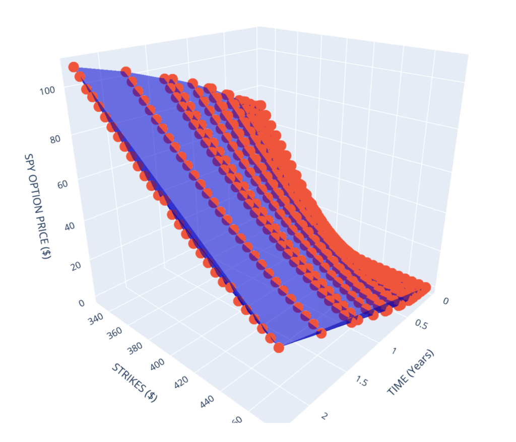
Using Plotly to graph 3D surface
First only looking at the Morning Price Surface
import plotly.graph_objects as go
from plotly.graph_objs import Surface
from plotly.offline import iplot, init_notebook_mode
init_notebook_mode()
fig = go.Figure(data=[go.Mesh3d(x=priceSurfaceMorn.maturity, y=priceSurfaceMorn.strike, z=priceSurfaceMorn.interpolation, color='mediumblue', opacity=0.55)])
fig.add_scatter3d(x=volSurfaceLongMorn.maturity, y=volSurfaceLongMorn.strike, z=volSurfaceLongMorn.price, mode='markers')
fig.update_layout(
    title_text='10:00 SPY Quoted Market Prices (Markers) vs 2d Interpolation (Mesh)',
    scene = dict(xaxis_title='TIME (Years)',
                    yaxis_title='STRIKES ($)',
                    zaxis_title='SPY OPTION PRICE ($)'),
    height=800,
    width=800
)
fig.show()
Plotting both the Morning and Afternoon Price Surfaces
import plotly.graph_objects as go
from plotly.graph_objs import Surface
from plotly.offline import iplot, init_notebook_mode
init_notebook_mode()
fig = go.Figure(data=[go.Mesh3d(x=priceSurfaceMorn.maturity, y=priceSurfaceMorn.strike, z=priceSurfaceMorn.interpolation, color='mediumblue', opacity=0.55),
                         go.Mesh3d(x=priceSurfaceArvo.maturity, y=priceSurfaceArvo.strike, z=priceSurfaceArvo.interpolation, color='red', opacity=0.55)])
# fig.add_scatter3d(x=volSurfaceLongMorn.maturity, y=volSurfaceLongMorn.strike, z=volSurfaceLongMorn.price, mode='markers')
fig.update_layout(
    title_text='10:00 vs 14:00 SPY Quoted Market Prices (Markers) vs 2d Interpolation (Mesh)',
    scene = dict(xaxis_title='TIME (Years)',
                    yaxis_title='STRIKES ($)',
                    zaxis_title='SPY OPTION PRICE ($)'),
    height=800,
    width=800
)
fig.show()
Calculation of Volatility Surface
Volatility array calculation from price_arr numpy array.
Create clean DataFrame for vol surface.
price_morn = 399.67
price_arvo = 396.75

s,m = np.meshgrid(strikes, maturity)
volatility_morn = implied_vol(price_morn_arr, K=s, t=m, S=price_morn, r=0.01, flag='c', q=0, return_as='numpy', on_error='ignore')
volatility_arvo = implied_vol(price_arvo_arr, K=s, t=m, S=price_arvo, r=0.01, flag='c', q=0, return_as='numpy', on_error='ignore')

vol_morn_arr = np.copy(volatility_morn)*100
vol_arvo_arr = np.copy(volatility_arvo)*100

vol_morn_arr[(vol_morn_arr < 1) | (vol_morn_arr > 120)] = np.nan
vol_arvo_arr[(vol_arvo_arr < 1) | (vol_arvo_arr > 120)] = np.nan

volSurfaceLongMorn['volatility'] = vol_morn_arr
volSurfaceLongArvo['volatility'] = vol_arvo_arr

volSurfaceLongMorn = volSurfaceLongMorn[~( (np.isnan(volSurfaceLongMorn['price'])) | (volSurfaceLongMorn['volatility']) > 60)]
volSurfaceLongArvo = volSurfaceLongArvo[~( (np.isnan(volSurfaceLongArvo['price'])) | (volSurfaceLongArvo['volatility']) > 60)]

vol_morn_arr = vol_morn_arr.reshape(np.shape(price_morn_arr))
vol_arvo_arr = vol_arvo_arr.reshape(np.shape(price_arvo_arr))

vol_morn_arr[price_morn_arr == np.nan] = np.nan
vol_arvo_arr[price_arvo_arr == np.nan] = np.nan

vol_morn_arr[:,0], vol_arvo_arr[:,0]
Interpolation using Bivariate Spline
Interpolation of volatility array using scipy’s SmoothBivariateSpline.
import scipy.interpolate as interpolate

s,m = s.flatten(),m.flatten()
vol_morn_arr,price_morn_arr = vol_morn_arr.flatten(), price_morn_arr.flatten()
vol_arvo_arr,price_arvo_arr = vol_arvo_arr.flatten(), price_arvo_arr.flatten()

mask_morn = np.isnan(vol_morn_arr)
mask_arvo = np.isnan(vol_arvo_arr)

sm,mm,vol_morn_arr,price_morn_arr = s[~mask_morn],m[~mask_morn],vol_morn_arr[~mask_morn], price_morn_arr[~mask_morn]
sa,ma,vol_arvo_arr,price_arvo_arr = s[~mask_arvo],m[~mask_arvo],vol_arvo_arr[~mask_arvo], price_arvo_arr[~mask_arvo]

kx, ky = 4, 4  # spline order
assert len(m) >= (kx+1)*(ky+1)

wm=np.abs(price_morn_arr - price_morn)/price_morn * np.sqrt(mm)
tck_morn = interpolate.SmoothBivariateSpline(mm, sm, vol_morn_arr, kx=kx, ky=ky, w=wm, bbox=[0, 5, 250, 650])

wa=np.abs(price_arvo_arr - price_arvo)/price_arvo * np.sqrt(ma)
tck_arvo = interpolate.SmoothBivariateSpline(ma, sa, vol_arvo_arr, kx=kx, ky=ky, w=wa, bbox=[0, 5, 250, 650])

strikes2 = np.linspace(strikes[0],strikes[-1],20)
maturity2 = np.linspace(maturity[0],maturity[-1],20)
s2,m2 = np.meshgrid(strikes2, maturity2)

vol_intpol_morn = tck_morn.ev(m2,s2)
vol_intpol_arvo = tck_arvo.ev(m2,s2)

# vol_intpol
Morning Volatility Surface Interpolation Displayed
Create DataFrame for plotting.
volSurfaceMorn2 = pd.DataFrame(vol_intpol_morn, index = maturity2, columns = strikes2)
volSurfaceLongMorn2 = volSurfaceMorn2.melt(ignore_index=False).reset_index()
volSurfaceLongMorn2.columns = ['maturity', 'strike', 'interpolation']

fig = go.Figure(data=[go.Mesh3d(x=volSurfaceLongMorn2.maturity, y=volSurfaceLongMorn2.strike, z=volSurfaceLongMorn2.interpolation, color='mediumblue', opacity=0.55)])
fig.add_scatter3d(x=volSurfaceLongMorn.maturity, y=volSurfaceLongMorn.strike, z=volSurfaceLongMorn.volatility, mode='markers')
fig.update_layout(
    title_text='Market Implied Volatility (Markers) vs 2d Interpolation (Mesh)',
    scene = dict(xaxis_title='TIME (Years)',
                    yaxis_title='STRIKES ($)',
                    zaxis_title='SPY IMPLIED VOL (%)'),
    height=800,
    width=800
)
fig.show()

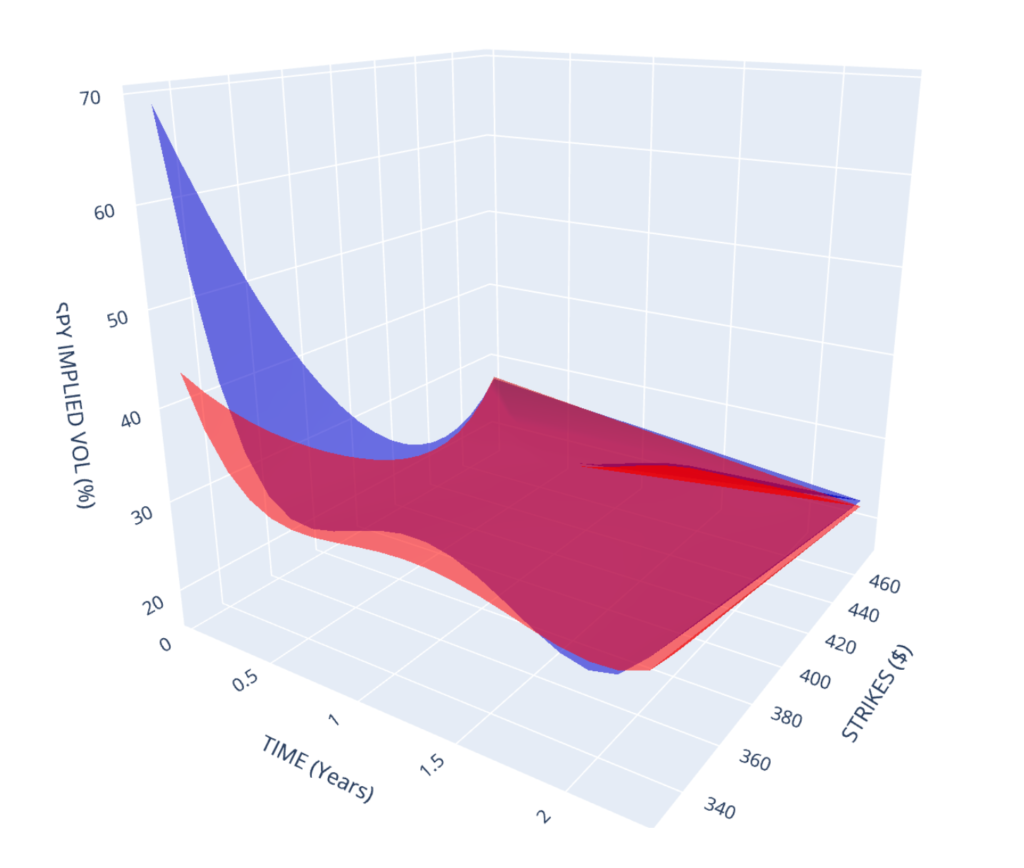
Morning vs Afternoon Vol Surfaces
volSurfaceArvo2 = pd.DataFrame(vol_intpol_arvo, index = maturity2, columns = strikes2)
volSurfaceLongArvo2 = volSurfaceArvo2.melt(ignore_index=False).reset_index()
volSurfaceLongArvo2.columns = ['maturity', 'strike', 'interpolation']

fig = go.Figure(data=[go.Mesh3d(x=volSurfaceLongMorn2.maturity, y=volSurfaceLongMorn2.strike, z=volSurfaceLongMorn2.interpolation, color='mediumblue', opacity=0.55, name='Morning'),
                     go.Mesh3d(x=volSurfaceLongArvo2.maturity, y=volSurfaceLongArvo2.strike, z=volSurfaceLongArvo2.interpolation, color='red', opacity=0.55, name='Afternoon')])
# fig.add_scatter3d(x=volSurfaceLongArvo.maturity, y=volSurfaceLongArvo.strike, z=volSurfaceLongArvo.volatility, mode='markers')

fig.update_layout(
    title_text='SPY Intraday Vol Surfaces 10:00 vs 14:00',
    scene = dict(xaxis_title='TIME (Years)',
                    yaxis_title='STRIKES ($)',
                    zaxis_title='SPY IMPLIED VOL (%)'),
    height=800,
    width=800,
    showlegend=True,
)
fig.show()