
Today we will be exploring the financial data structures as discussed in Advances in Financial Machine Learning by Prof. Marcos Lopez de Prado [2018].
Table 2.1 The Four Essential Types of Financial Data
| Fundamental Data | Market Data | Analytics | Alternative Data |
| Assets | Price/yield/implied volatility | Analyst recommendations | Satellite/CCTV imagesLiabilities |
| Liabilities | Volume | Credit Ratings | Google searchers |
| Earnings expectations | Dividend/coupons | Earnings expectations | Twitter/chats |
| Cost/earnings | Open interest | News sentiment | Meta data |
| Macro variables | Quotes/cancellations |
Standard Bars for Financial Machine Learning
- Time Bars
- Tick Bars
- Volume Bars
- Dollar Bars
First let’s import our dependencies.
Import the course of sales or trade tick information. Here I only have access to one day’s worth of trade history freely provided by my broker CommSec.
import pandas as pd
import numpy as np
import matplotlib.pyplot as plt
import datetime as dt

trades = pd.read_csv('https://raw.githubusercontent.com/ASXPortfolio/jupyter-notebooks-data/main/CBA_trades.csv')
trades.head()
Now we need to transform the trade pandas dataframe into a format with datetime as the index. Look at volume of trades vs time.
trades.Time = pd.to_datetime(trades.Time)
trades.set_index('Time', inplace=True)
trades.plot()
Apply mask of only market open hours
mask = (trades.index > dt.datetime(2021,6,10,10,0,0)) & (trades.index <= dt.datetime(2021,6,10,16,0,0))
trades_mh = trades.iloc[mask]
trades_mh.head()
1. Time Bars
Time bars are obtained by sampling information at fixed intervals e.g. once every 5 minutes.
time_bars = trades_mh.groupby(pd.Grouper(freq='1min')).agg({'Price $': 'ohlc', 'Volume': 'sum'})
time_bars_price = time_bars.loc[:, 'Price $']
time_bars_price

time_bars = np.log(time_bars_price.close/time_bars_price.close.shift(1)).dropna()

bin_len = 0.001
plt.hist(time_bars, bins=np.arange(min(time_bars),max(time_bars)+bin_len, bin_len))
plt.show()
What are the Issues?
– oversampling information from low activity periods
– undersampling information from high-activity periods
– Time sampled data often have poor statistical properties (Easley, Lopez de Prado, and O’Hara [2011]):
– serial correlation: correlation of data with a delayed copy of itself (lag)
– heteroschedasticity: variance (residual term variation/error) changes over time
– nonnormality of returns
This can cause issues in our Analysis:
– Autocorrelation can cause problems in conventional analyses (such as ordinary least squares regression) that assume independence of observations.
– Heteroscedasticity is a problem because ordinary least squares (OLS) regression assumes that all residuals are drawn from a population that has a constant variance (homoscedasticity).
GARCH models were developed to deal with heteroschedasticity. By sampling price and volume information as a subordinated process of trading activity we can avoid this problem to begin with.
Helper bar function to construct / return a integer number of bars.
def bar(x, y):
    return np.int64(x/y)*y
2. Tick Bars
The sample variables Open, High, Low, Close and Volume are sampled over a pre-defined number of transactions.
transactions = 75

tick_bars = trades_mh.groupby(bar(np.arange(len(trades_mh)), transactions)).agg({'Price $': 'ohlc', 'Volume': 'sum'})
tick_bars_price = tick_bars.loc[:, 'Price $']
tick_bars_price

tick_bars = np.log(tick_bars_price.close/tick_bars_price.close.shift(1)).dropna()

bin_len = 0.0001
plt.hist(tick_bars, bins=np.arange(min(tick_bars),max(tick_bars)+bin_len, bin_len))
plt.show()
3. Volume Bars
Volume bars are sampled every time a pre-defined amount the the security’s units have been exchanged.
traded_volume = 10000

volume_bars = trades_mh.groupby(bar(np.cumsum(trades_mh['Volume']), traded_volume)).agg({'Price $': 'ohlc', 'Volume': 'sum'})
volume_bars_price = volume_bars.loc[:,'Price $']
volume_bars_price

volume_bars = np.log(volume_bars_price.close/volume_bars_price.close.shift(1)).dropna()

bin_len = 0.0001
plt.hist(volume_bars, bins=np.arange(min(volume_bars),max(volume_bars)+bin_len, bin_len))
plt.show()
4. Dollar Bars
Dollar bars are formed by sampling an observation every time a pre-defined market value is exchanged.
market_value = 700000

dollar_bars = trades_mh.groupby(bar(np.cumsum(trades_mh['Value $']), market_value)).agg({'Price $': 'ohlc', 'Volume':'sum'})
dollar_bars_price = dollar_bars.loc[:,'Price $']
dollar_bars_price

dollar_bars = np.log(dollar_bars_price.close/dollar_bars_price.close.shift(1)).dropna()

bin_len = 0.0001
plt.hist(dollar_bars, bins=np.arange(min(dollar_bars),max(dollar_bars)+bin_len, bin_len))
plt.show()
Plot Distributions
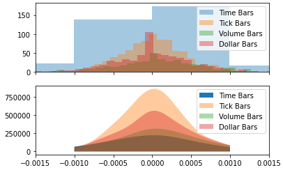
import matplotlib.pyplot as plt
import numpy as np
from scipy import stats
import seaborn as sns

cdmx_edad = np.random.normal(0, 20,10000)+10
ed_sup_edad = dollar_bars

dollar_bars = np.log(dollar_bars_price.close/dollar_bars_price.close.shift(1)).dropna()
volume_bars = np.log(volume_bars_price.close/volume_bars_price.close.shift(1)).dropna()
tick_bars = np.log(tick_bars_price.close/tick_bars_price.close.shift(1)).dropna()
time_bars = np.log(time_bars_price.close/time_bars_price.close.shift(1)).dropna()


fig, (ax1, ax2) = plt.subplots(nrows=2, sharex=True)
# bins = np.arange(10,61,1)
bin_len = 0.001
ax1.hist(time_bars, bins=np.arange(min(time_bars),max(time_bars)+bin_len, bin_len),alpha=0.4, label='Time Bars')
bin_len = 0.0001
ax1.hist(tick_bars, bins=np.arange(min(tick_bars),max(tick_bars)+bin_len, bin_len),alpha=0.4, label='Tick Bars')
ax1.hist(volume_bars, bins=np.arange(min(volume_bars),max(volume_bars)+bin_len, bin_len),alpha=0.4, label='Volume Bars')
ax1.hist(dollar_bars, bins=np.arange(min(dollar_bars),max(dollar_bars)+bin_len, bin_len),alpha=0.4, label='Dollar Bars')

ax1.legend()

dollar_bars_kde = stats.gaussian_kde(dollar_bars)
tick_bars_kde = stats.gaussian_kde(tick_bars)
volume_bars_kde = stats.gaussian_kde(volume_bars)
time_bars_kde = stats.gaussian_kde(time_bars)

x = np.linspace(-0.001,0.001,500)
dollar_bars_curve = dollar_bars_kde(x)*dollar_bars.shape[0]
tick_bars_curve = tick_bars_kde(x)*tick_bars.shape[0]
volume_bars_curve = volume_bars_kde(x)*volume_bars.shape[0]
time_bars_curve = time_bars_kde(x)*time_bars.shape[0]

# ax2.plot(x, cdmx_curve, color='r')
ax2.fill_between(x, 0, time_bars_curve, alpha=1, label='Time Bars')
ax2.fill_between(x, 0, tick_bars_curve, alpha=0.4, label='Tick Bars')
ax2.fill_between(x, 0, volume_bars_curve, alpha=0.4, label='Volume Bars')
ax2.fill_between(x, 0, dollar_bars_curve, alpha=0.4, label='Dollar Bars')

ax1.set_xlim(-0.0015,0.0015)

# ax2.plot(x, ed_sup_curve, color='b')
ax2.legend()
plt.show()

len_tick_bars =  np.arange(min(tick_bars),max(tick_bars)+bin_len, bin_len)
len(len_tick_bars)
sns.kdeplot(dollar_bars, gridsize=1000, shade=True, label='Dollar Bars')
sns.kdeplot(volume_bars, gridsize=1000, shade=True, label='Volume Bars')
sns.kdeplot(tick_bars, gridsize=25, shade=True, label='Tick Bars')
sns.kdeplot(time_bars, gridsize=50, shade=True, label='Time Bars')

plt.xlim(-0.0025,0.0025)

plt.xlabel('Log Returns (%)')
plt.ylabel('Frequency')
plt.title('KDE of Standard Price & Volume Bars')

# dollar_bars = np.log(dollar_bars_price.close/dollar_bars_price.close.shift(1)).dropna()
# volume_bars = np.log(volume_bars_price.close/volume_bars_price.close.shift(1)).dropna()
# tick_bars = np.log(tick_bars_price.close/tick_bars_price.close.shift(1)).dropna()
# time_bars = np.log(time_bars_price.close/time_bars_price.close.shift(1)).dropna()
# sns.kdeplot(eduacion_superior['EDAD'], shade=True)