Background
The Goal:
Identify information based trading activity.
What does that mean?
Informed traders of good news will profit by buying while traders with bad news will profit by selling.
Motivation: Why we Care?
According to market microstructure models, trade data has historically played a key role because of its signal value for underlying private information [1].
For example, trade imbalance between buys and sells can signal liquidity pressue and lead to subsequent price movements. This can be cause by informed traders transacting in large volumes. Therefore, we want to detect informative trade flow!
By identifying informed trading activity, this can help characterise investor behaviour and participants / market makers can adjust accordingly.
Though information detection is of primary importance, aggressor-signing can be useful as well for assessing trading costs, and an ideal algorithm should do both [2].
Traditional Approaches:
In the past, emphasis was placed on attempting to identify individual trade’s aggressor: in other words, was this trade initiated by the buyer or the seller. Some exchanges make this information available within their data streams, but many do not.
The established methods, most notably the algorithms of Lee and Ready (1991) (LR), Ellis et al. (2000) (EMO) and Chakrabarty et al. (2007) (CLNV), classify trades based on the proximity of the transaction price to the quotes in effect at the time of the trade.
In today’s market, this is problematic due to the increased frequency of order submission and cancellation, across many exchanges.
Problem:
The complications of using these historical algorithms to assess the agressor side of trading is very difficult in the world of high frequency markets.
In the new world of electronic markets, there are:
- complex order types: for example hidden orders
- market fragmentation: trading is split across many exchanges and alternative trading venues. These appear on the consolidated tape but at different latencies.
- high frequency of order cancellations: as much as up to 98% [1] therefore complicating actual quotes at time of trades
- complex order execution algorithms: execution algorithms that can chop “parent orders” into numerous “child” orders distribute them across exchanges with different order types
In summary trades on the consolidated tape can be out of order and with order cancellation rates up to 98% this complicates knowing actual quotes at the time of trades.
Trade classification algorithms that rely on the following, can be severly compromised:
- rules based on up-ticks or down-ticks
- proximity to bid and ask quotes
Both research papers Easley et al. (2016) [1] and Panayides et al.(2019) [2] found that traditional algorithms that find individual trade agressor no longer captures information.
- Traditional algorithms fail to explain the dynamics, of spreads or prices over time.
- This suggests that the other sources of buying (or selling) pressure ignored by the tick rule are so important that the tick rule does not succeed in detecting the informational
content carried by the order flow. (sourced: directly from [1])
Solution:
Easley et al. (2012) created the Bulk Volume Classification (BVC) algorithm, which instead of classifying individual trades, aggregates trades by volume or ticks to then infer the buying and selling activity within these collective groups of trades. The BVC algorithm therefore focussing on classification of aggregated trade flows, which both [1] & [2] have found to be better linked to proies of informed-based trading.
Because BVC uses the market makers’ aggregated response to order flow to infer its informational content, it overcomes these limitations of the tick rule and
provides a new tool for discerning the presence of underlying information from market data (sourced: directly from [1]).
Both [1] & [2] find that BVC can identify trade aggressors as well as traditional algorithms, and its signed order flow is the only measure that is reliably related to different illiquidity measures shown to capture the trading intensions of informed traders.
Methodology: Scientific Method [1] & [2] – only for those interested:
Theory in market microstructure predicts that with more informed trading, liquidity is affected as market makers widen spreads to protect themselves [2].
Easley et al. (2012) therefore argued that if an algorithm is capturing underlying information, then absolute order imbalance should be positively related to spread in bar \(\tau\) [2].
Both [1] & [2] ran regression on various spread estimates on estimated order imbalance and lagged spread estimates:
$$\large Spread_\tau = \alpha_0 + \alpha_1 [Spread_{\tau-1}] + \gamma [\hat{OI}\tau] +\epsilon\tau$$
where estimated absolute order imbalance (\(\hat{OI}_\tau\)) is defined as:
\(\large |\hat{OI}\tau| = |\frac{\hat{V}\tau^B – \hat{V}\tau^S}{V\tau}| = |2 \frac{\hat{V}\tau^B}{V\tau} – 1 |\)
and \(\hat{V}\tau^B and \hat{V}\tau^S\) are estimated buy and sell volumes respectively within a bar \(\tau\)
Our AIM:
Implement the BVC algorithm using ThetaData historical data.
In future videos, I plan to adapt this to include realtime streaming assessment. Also I plan on creating a series that focuses on developing a market making trading bot that can could incorperate this information as a risk managment strategy.
References:
import os
import time
import pickle

import random
import numpy as np
import pandas as pd
import matplotlib.pyplot as plt

from datetime import timedelta, datetime, date
from thetadata import ThetaClient, OptionReqType, OptionRight, StockReqType, DateRange, DataType, TradeCondition, Exchange
1. Getting the Data
ThetaData is an incredible API where we can request realtime streaming of NBBO options data, or request historical options data (trades & quotes) back for 10 years.
1.1 Get Option Expirations on particular Underlying
from dotenv import load_dotenv
load_dotenv()

your_username = os.environ['thetadata_username']
your_password = os.environ['thetadata_password']

def get_expirations(root_ticker) -> pd.DataFrame:
    """Request expirations from a particular options root"""
    # Create a ThetaClient
    client = ThetaClient(username=your_username, passwd=your_password, jvm_mem=4, timeout=15)

    # Connect to the Terminal
    with client.connect():

        # Make the request
        data = client.get_expirations(
            root=root_ticker,
        )

    return data


root_ticker = 'MSFT'
expirations = get_expirations(root_ticker)
expirations
1.2 Get all Strikes for each MSFT Option Expiry
We will need these later, so I will build up a dictionary and pickle this data for future use.
def get_strikes(root_ticker, expiration_dates) -> dict:
    """Request strikes from a particular option contract"""
    # Create a ThetaClient
    client = ThetaClient(username=your_username, passwd=your_password, jvm_mem=4, timeout=15)

    all_strikes = {}

    # Connect to the Terminal
    with client.connect():

        for exp_date in expiration_dates:

            # Make the request
            data = client.get_strikes(
                root=root_ticker,
                exp=exp_date
            )

            all_strikes[exp_date] = pd.to_numeric(data)


    return all_strikes

root_ticker = 'MSFT'

all_strikes = get_strikes(root_ticker, expirations)

with open('MSFT_strikes.pkl', 'wb') as f:
    pickle.dump(all_strikes, f)

with open('MSFT_strikes.pkl', 'rb') as f:
    all_strikes = pd.read_pickle(f)

all_strikes[expirations[360]]
1.3 Pre-processing Expirations for actively traded
Market-Makers are not forced to show Quotes on all options!
There are rules listed for each Exchange that market makers must abide by. For Example on the NASDAQ where MSFT trades here are the rules
Specifically there is a large difference between the obligation of a Competitive Market Maker and the Primary Market Makers for a particular options series. This is notable in whether they need to present two-sided quotes on Non-standard options like weekly or quarterly expiry options and adjusted options.
To be safe here, we will only want to return option contracts with ‘standard’ option expires. These expire on the Saturday following the third Friday of the month, and some have the expiry date as the Third friday of the month, but in the past were recorded as the Saturday. Therefore we need to find the intersection of all the expiries that Thetadata has options data for and the 3rd Fridays and the following Saturday dates for every month since Jun-2021.
def get_mth_expirations(expirations: pd.Series) -> pd.Series:
    trading_days = pd.date_range(start=datetime(2012,6,1),end=datetime(2023,11,14),freq='B')
    # The third friday in every month
    contracts1 = pd.date_range(start=datetime(2012,6,1),end=datetime(2024,12,31),freq='WOM-3FRI')
    # Saturday following the third friday in every month
    contracts2 = pd.date_range(start=datetime(2012,6,1),end=datetime(2022,12,31),freq='WOM-3FRI')+timedelta(days=1)
    # Combine these contracts into a total pandas index list
    contracts = contracts1.append(contracts2)
    # Find contract expiries that match with ThetaData expiries
    mth_expirations = [exp for exp in expirations if exp in contracts]
    # Convert from python list to pandas datetime
    mth_expirations = pd.to_datetime(pd.Series(mth_expirations))
    # print information of processed expiration data
    print('Number of possible monthly contracts', len(contracts), 'compared to total avail',len(mth_expirations),
      'compared to total no. options avail (incl. quarterly + weekly)', len(expirations))
    return mth_expirations

mth_expirations = get_mth_expirations(expirations)
1.4 Get all trade data for particular contract and strikes
Now we have a list of possiblte options contracts and their corresponding strikes.
We need a function that allows us to request trades for particular contract across a number of strikes.
# Make the request
def get_option_trades(root_ticker, exp_date, strikes, start_date, end_date, interval_size=0, opt_type=OptionRight.CALL) -> pd.DataFrame:
    """Request trades for particular contract across a number of strikes"""
    # Create a ThetaClient
    client = ThetaClient(username=your_username, passwd=your_password, jvm_mem=12, timeout=30)

    # Store all iv in datas dictionary
    datas = {}

    # Connect to the Terminal
    with client.connect():

        # For each expiry we want to get closest ATM iv
        for strike in strikes:

            try:
                # Attempt to request historical options implied volatility
                data = client.get_hist_option(
                    req=OptionReqType.TRADE_QUOTE,
                    root=root_ticker,
                    exp=exp_date,
                    strike=strike,
                    right=opt_type,
                    date_range=DateRange(start_date, end_date),
                    progress_bar=False,
                    interval_size=interval_size
                )

                # Store data in dictionary
                datas[strike] = data

            except Exception as e:
                # If unavailable, store np.nan
                datas[strike] =  np.nan
                print(e)

    return datas


exp_date = mth_expirations[130]
strikes = all_strikes[exp_date].tolist()

print('expiry date:\n', exp_date, '\n')
print('strikes:\n', strikes)

root_ticker = 'MSFT'
start_date = datetime(2023,1,1)
end_date = datetime(2023,6,6)

trades = get_option_trades(root_ticker, exp_date, strikes, start_date, end_date)

with open('trades.pkl', 'wb') as f:
    pickle.dump(trades, f)


with open('trades.pkl', 'rb') as f:
    trades = pd.read_pickle(f)

for k, v in trades.items():
    print(k, 0 if np.isnan(v).any().any() else len(v))

trades_df = trades[300.0]
trades_df
Include Trade Types
Include ENUM names for Trade Condition Column
trade_cond = {x.value : x.name for x in TradeCondition}
exchanges = {x.value[0] : x.name for x in Exchange}
trades_df['Condition'] = trades_df.apply(lambda row: trade_cond[row[DataType.CONDITION]] if row[DataType.CONDITION] in trade_cond.keys() else trade_cond[-row[DataType.CONDITION]], axis=1)
trades_df.groupby('Condition').agg({DataType.SIZE: 'sum'})

trades_df['BID_EXCHANGE'] = trades_df.apply(lambda row: exchanges[row[DataType.BID_EXCHANGE]] if row[DataType.BID_EXCHANGE] in exchanges.keys() else exchanges[-row[DataType.BID_EXCHANGE]], axis=1)
trades_df['ASK_EXCHANGE'] = trades_df.apply(lambda row: exchanges[row[DataType.ASK_EXCHANGE]] if row[DataType.ASK_EXCHANGE] in exchanges.keys() else exchanges[-row[DataType.ASK_EXCHANGE]], axis=1)
trades_df.groupby(['BID_EXCHANGE']).agg({DataType.SIZE: 'sum'})

trades_df = trades_df.drop(columns=[DataType.MS_OF_DAY, DataType.MS_OF_DAY2, DataType.SEQUENCE, DataType.CONDITION, DataType.BID_EXCHANGE, DataType.ASK_EXCHANGE])
trades_df
2. Bulk Volume Classification
2.1 The Algorithm
A (time / volume) bar \(\Large \tau\) is assigned the price change \(\Delta P = P_\tau – P_{\tau-1}\), let:
$$\large \hat{V}\tau^B = V\tau \times t(\frac{\Delta P}{\sigma_{\Delta P}}, df)$$
$$\large \hat{V}\tau^S = V\tau \times \left[ 1 – t(\frac{\Delta P}{\sigma_{\Delta P}}, df) \right]$$
Here \(V_\tau\) is the volume traded during bar \(\tau\) which we would like to classify into Buy (\(\hat{V}\tau^B\)) and Sell (\(\hat{V}\tau^S\)) volumes.
Most importantly, \(t\) is the CDF of Student’s t distribution, with \(df\) degrees of freedom.
The formula I will use for volume-weighted standard deviation of price changes is:
$$\large \sigma_{\Delta P} = \sqrt{\frac{\sum^n_{\tau=1} V_\tau (\Delta P_\tau – \overline{\Delta P})^2}{\sum^n_{\tau=1} V_\tau}} $$
This is consistent with Panayides, Shohfi and Smith (2019). We will also perform the analysis using 0.25 degrees of freedom for the student t disribution following Easley, Lopez de Prado and O’Hara (2016) baseline approach.
2.2 Examples:
Volumes are therefore assigned by direction of price changes and magnitude.
Volumes will be weighted depending on how large the price change in absolute terms (magnitude) is relative to the distribution of price changes.
\(\Delta P \sim 0\): If there is no price change The total volume traded will be split equally between buy and sell volume. \(\Delta P > 0\): If price increases Volume is weighted more towards buys than sells. \(\Delta P < 0\): If price decreases Volume is weighted more towards sells than buys.
2.3 Writing the functions
import scipy as sc

def std_dev(price_diff: pd.Series, n: int):
    if len(price_diff) < n:
        raise ValueError(f'Lookback window is greater than rows of dataframe ({len(price_diff)})')
    else:
        return price_diff.rolling(window=n).std()

def bulk_volume_classifier(ohlc_vol_bars: pd.DataFrame, lookback: int, df: float = 0.25) -> pd.DataFrame:
    """Classify's traded volume into fraction of buy's and sell's

    Algorithm: Bulk Volume Classification created by Easley, Lopez de Prado and O'Hara (2016)

    Args:
        bar_ohlc_vol (pd.DataFrame): price bar with ohlc and volume data
        lookback (int): number of lookback bars used for standard deviation calculation
        df (int): degrees of freedom within the Student t distribution

    Returns:
        pd.DataFrame: fraction of buys vs sells per price bar normalised between [-1,1]

    """
    # calculate deltaP and sigmaP
    deltaP = ohlc_vol_bars.close-ohlc_vol_bars.close.shift(1)
    sigmaP = std_dev(price_diff=deltaP, n=lookback)
    # z variable for student t-distribution
    z = deltaP/sigmaP
    # weighted
    x = sc.stats.t.cdf(z,df)
    # calculate Vb_hat, Vs_hat individually
    Vb_hat = ohlc_vol_bars.volume * x
    Vs_hat = ohlc_vol_bars.volume * (1-x)
    # rename pd.Series before concatinating
    Vb_hat.name = 'V_buy'
    Vs_hat.name = 'V_sell'
    # combine pd.Series and create pd.DataFrame
    res = pd.concat([Vb_hat, Vs_hat], axis=1)
    # this is the frac of buys to total volume traded
    res['V_frac'] = x
    return res
2.4 Tick Bars & Volume Bars
Creating Helper bar functions, will allow us to construct / return a integer number of bars.
def bar(x, y):
    return np.int64(x/y)*y
Tick Bars
The sample variables Open, High, Low, Close and Volume are sampled over a pre-defined number of transactions.
def create_tick_bars(trades: pd.DataFrame, transactions: int) -> pd.DataFrame:
    tick_bars_raw = trades.groupby(bar(np.arange(len(trades)), transactions)).agg({DataType.PRICE: 'ohlc', DataType.SIZE: 'sum'})
    tick_bars = tick_bars_raw.loc[:,DataType.PRICE]
    tick_bars['volume'] = tick_bars_raw.loc[:,DataType.SIZE]
    return tick_bars

no_transactions = 20
tick_bars = create_tick_bars(trades_df, no_transactions)

tick_bars_plot = np.log(tick_bars.close/tick_bars.close.shift(1)).dropna()
bin_len = 0.01
plt.hist(tick_bars_plot, bins=np.arange(min(tick_bars_plot),max(tick_bars_plot)+bin_len, bin_len))
plt.show()
Volume Bars
Volume bars are sampled every time a pre-defined amount the the security’s units have been exchanged.
def create_volume_bars(trades: pd.DataFrame, volume: int) -> pd.DataFrame:
    volume_bars_raw = trades.groupby(bar(np.cumsum(trades[DataType.SIZE]), volume)).agg({DataType.PRICE: 'ohlc', DataType.SIZE: 'sum'})
    volume_bars = volume_bars_raw.loc[:,DataType.PRICE]
    volume_bars['volume'] = volume_bars_raw.loc[:,DataType.SIZE]
    return volume_bars

traded_volume = 10
volume_bars = create_volume_bars(trades_df, traded_volume)

volume_bars_plot = np.log(volume_bars.close/volume_bars.close.shift(1)).dropna()
bin_len = 0.01
plt.hist(volume_bars_plot, bins=np.arange(min(volume_bars_plot),max(volume_bars_plot)+bin_len, bin_len))
plt.show()
3. Classifying Trades using BVC
3.1 Running the algorithm
Our function takes either tick or volume bars to classify volumes. The number of transactions or traded volume can be individually specified.
no_transactions = 5
tick_bars = create_tick_bars(trades_df, no_transactions)

traded_volume = 5
volume_bars = create_volume_bars(trades_df, traded_volume)

bvc = bulk_volume_classifier(ohlc_vol_bars=tick_bars, lookback=100)
bvc.loc[:,'close'] = tick_bars.close

bvc
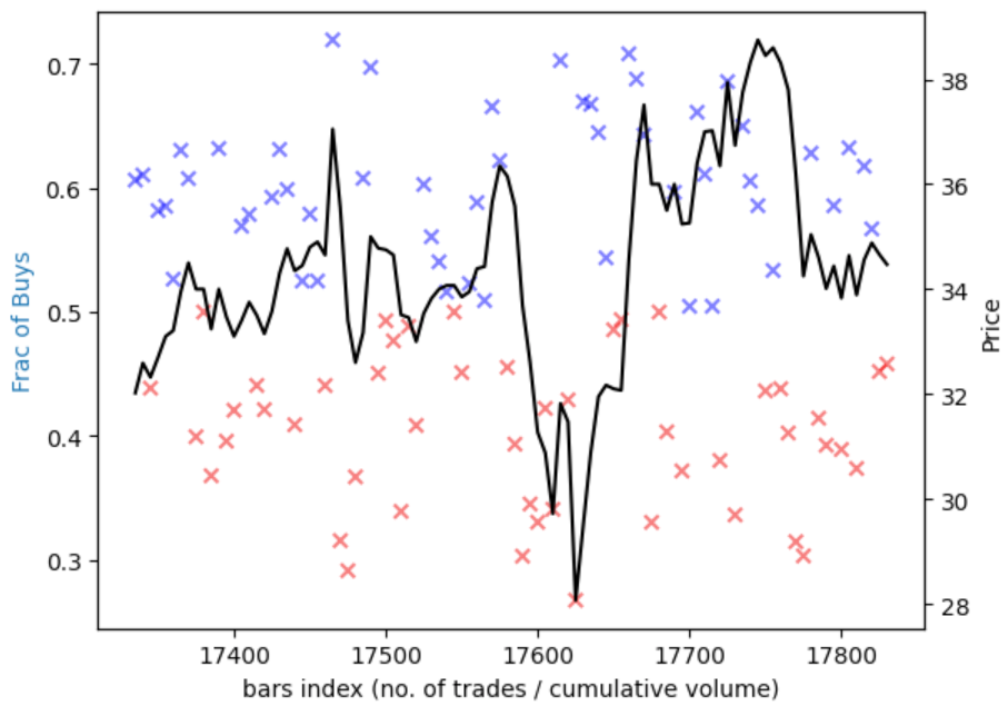
3.2 Visualising our Results
Let’s just a subset of the data.
subset = 100

fig, ax1 = plt.subplots()
ax2 = ax1.twinx()
ax1.scatter(bvc.index[-subset:], bvc.V_frac[-subset:], marker='x', color=np.where(bvc.V_frac[-subset:]>0.5, 'blue', 'red'), alpha=0.5)
ax2.plot(tick_bars.close[-subset:], 'k')

ax1.set_xlabel('bars index (no. of trades / cumulative volume)')
ax1.set_ylabel('Frac of Buys', color='tab:blue')
ax2.set_ylabel('Price', color='k')

plt.show()
3.3 Creating an Indicator
def create_indicator(arr: np.ndarray) -> np.ndarray:
    """Takes numpy array [0,1] and normalises values between [-1,1]"""
    return 2 * arr - 1

def moving_average(indicator: pd.Series, n: int) -> pd.Series:
    """Takes indicator every time period, provides moving average"""
    return indicator.rolling(window=n).mean()

bvc['indicator'] = create_indicator(bvc.V_frac)
bvc['ma10'] = moving_average(bvc.indicator, 10)
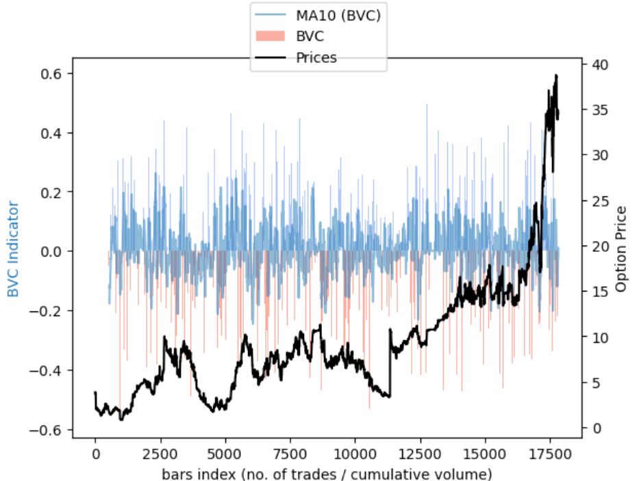
3.4 Cleaning up our findings
subset = 10000

bvc_subset = bvc[-subset:]

fig, ax1 = plt.subplots()
# plot line chart on axis #1

ax1.bar(bvc_subset.index, bvc_subset.indicator, label='BVC', width=no_transactions, alpha=0.5, color=np.where(bvc_subset.indicator[-subset:]>0, 'cornflowerblue', 'tomato'))
ax1.plot(bvc_subset.index, bvc_subset.ma10, label='MA10 (BVC)', alpha=0.5)
# set up the 2nd axis
ax2 = ax1.twinx()
# plot bar chart on axis #2
ax2.plot(bvc_subset.index, bvc_subset.close, 'k-', label='Prices')
ax2.grid(False) # turn off grid #2

ax1.set_xlabel('bars index (no. of trades / cumulative volume)')
ax1.set_ylabel('BVC Indicator', color='tab:blue')
ax2.set_ylabel('Option Price', color='k')

fig.legend(loc=9)

plt.show()