Historical Volatility & Risk-Return Measures

In this tutorial we compute and track historical volatility over time.

import datetime as dt
import pandas as pd
import numpy as np

from pandas_datareader import data as pdr
import plotly.offline as pyo
import plotly.graph_objects as go
from plotly.subplots import make_subplots

pyo.init_notebook_mode(connected=True)
pd.options.plotting.backend = 'plotly'

Get stock data with pandas_datareader

end = dt.datetime.now()
start = dt.datetime(2015,1,1)

df = pdr.get_data_yahoo(['^AXJO', 'CBA.AX','NAB.AX','STO.AX','WPL.AX'], start, end)
Close = df.Close
Close.head()

Compute log returns

log_returns = np.log(df.Close/df.Close.shift(1)).dropna()
log_returns

Calculate daily standard deviation of returns

daily_std = log_returns.std()

annualized_std = daily_std * np.sqrt(252)
annualized_std

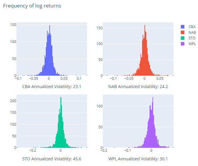
Plot histogram of log returns with annualized volatility

fig = make_subplots(rows=2, cols=2)

trace0 = go.Histogram(x=log_returns['CBA.AX'], name='CBA')
trace1 = go.Histogram(x=log_returns['NAB.AX'], name='NAB')
trace2 = go.Histogram(x=log_returns['STO.AX'], name='STO')
trace3 = go.Histogram(x=log_returns['WPL.AX'], name='WPL')

fig.append_trace(trace0, 1, 1)
fig.append_trace(trace1, 1, 2)
fig.append_trace(trace2, 2, 1)
fig.append_trace(trace3, 2, 2)

fig.update_layout(autosize = False, width=700, height=600, title='Frequency of log returns',
                  xaxis=dict(title='CBA Annualized Volatility: ' + str(np.round(annualized_std['CBA.AX']*100, 1))),
                  xaxis2=dict(title='NAB Annualized Volatility: ' + str(np.round(annualized_std['NAB.AX']*100, 1))),
                  xaxis3=dict(title='STO Annualized Volatility: ' + str(np.round(annualized_std['STO.AX']*100, 1))),
                  xaxis4=dict(title='WPL Annualized Volatility: ' + str(np.round(annualized_std['WPL.AX']*100, 1))))

fig.show()

TRADING_DAYS = 60
volatility = log_returns.rolling(window=TRADING_DAYS).std()*np.sqrt(TRADING_DAYS)
volatility.tail()

volatility.plot().update_layout(autosize = False, width=600, height=300).show()

Sharpe ratio

The Sharpe ratio which was introduced in 1966 by Nobel laureate William F. Sharpe is a measure for calculating risk-adjusted return. The Sharpe ratio is the average return earned in excess of the risk-free rate per unit of volatility.

Rf = 0.01/255
sharpe_ratio = (log_returns.rolling(window=TRADING_DAYS).mean() - Rf)*TRADING_DAYS / volatility

sharpe_ratio.plot().update_layout(autosize = False, width=600, height=300).show()

Sortino Ratio

The Sortino ratio is very similar to the Sharpe ratio, the only difference being that where the Sharpe ratio uses all the observations for calculating the standard deviation the Sortino ratio only considers the harmful variance.

sortino_vol = log_returns[log_returns<0].rolling(window=TRADING_DAYS, center=True, min_periods=10).std()*np.sqrt(TRADING_DAYS)
sortino_ratio = (log_returns.rolling(window=TRADING_DAYS).mean() - Rf)*TRADING_DAYS / sortino_vol

sortino_vol.plot().update_layout(autosize = False, width=600, height=300).show()

sortino_ratio.plot().update_layout(autosize = False, width=600, height=300).show()

Modigliani ratio (M2 ratio)

The Modigliani ratio measures the returns of the portfolio, adjusted for the risk of the portfolio relative to that of some benchmark.

m2_ratio = pd.DataFrame()

benchmark_vol = volatility['^AXJO']
for c in log_returns.columns:
    if c != '^AXJO':
        m2_ratio[c] = (sharpe_ratio[c]*benchmark_vol/TRADING_DAYS + Rf)*TRADING_DAYS

m2_ratio.plot().update_layout(autosize = False, width=600, height=300).show()

Max Drawdown

Max drawdown quantifies the steepest decline from peak to trough observed for an investment. This is useful for a number of reasons, mainly the fact that it doesn’t rely on the underlying returns being normally distributed.

def max_drawdown(returns):
    cumulative_returns = (returns+1).cumprod()
    peak = cumulative_returns.expanding(min_periods=1).max()
    drawdown = (cumulative_returns/peak)-1
    return drawdown.min()


returns = df.Close.pct_change()
max_drawdowns = returns.apply(max_drawdown, axis=0)
max_drawdowns*100

Calmar Ratio

Calmar ratio uses max drawdown in the denominator as opposed to standard deviation.

calmars = np.exp(log_returns.mean()*255)/abs(max_drawdowns)
calmars.plot.bar().update_layout(autosize = False, width=600, height=300).show()