
The Efficient Frontier is a common phrase in Modern Finance since the inception of Modern Portfolio Theory in 1952 by Harry Markowitz.
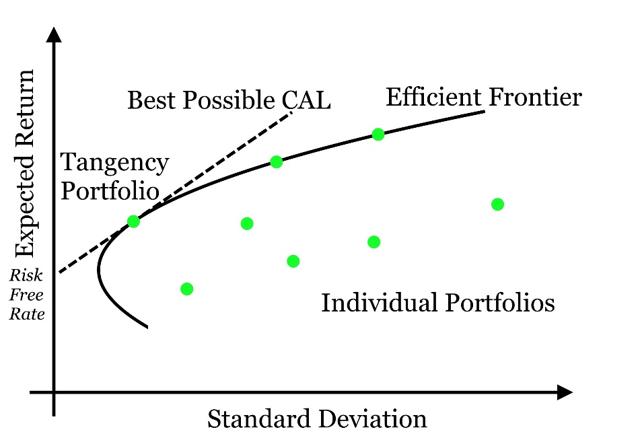
Intro to the Efficient Frontier
First step is to import data, this will be done by utilising the pandas_datareader module which has access to yahoo finance data. After importing the data, we are only interested in the Closing Prices for the day and hence drop all other columns from the dataframe to make it easier to work with.
By transforming the dataframe to daily percentage changes, we are able to calculate the covariance between assets and the mean daily returns with ease.
# Import data
def getData(stocks, start, end):
    stockData = pdr.get_data_yahoo(stocks, start=start, end=end)
    stockData = stockData['Close']

    returns = stockData.pct_change()
    meanReturns = returns.mean()
    covMatrix = returns.cov()
    return meanReturns, covMatrix
Now, we aren’t concerned with the individual performance of stocks – that’s something we can all just look up online. No, what we are interested in is the performance of either Our Own Portfolio or an Optimised Portfolio. For example we may have a portfolio with the following allocations:
- 30% weighting in BHP;
- 30% weighting in CBA; and,
- 40% weighting in TLS.
In order to determine the portfolio’s performance or characterisitics over a given period of time, we will need to calculate these metrics with another function called portfolioPerformance.
def portfolioPerformance(weights, meanReturns, covMatrix):
    returns = np.sum(meanReturns*weights)*252
    std = np.sqrt(
            np.dot(weights.T,np.dot(covMatrix, weights))
           )*np.sqrt(252)
    return returns, std
Maximium Sharpe Ratio Portfolio
Owning a portfolio with the Maximium Sharpe Ratio is the dream of every investor, “or more likely should be”!!!
So what is the dream portfolio and how can you make one?
Well unfortunately no one has a crystal ball, if we did we would be asking the investment gods what each assets return and variance is going to be into the future and minimise risk while maximising our return. So we have to estimate these parameters, and one way of doing this is using historical stock price data.
def negativeSR(weights, meanReturns, covMatrix, riskFreeRate = 0):
    pReturns, pStd = portfolioPerformance(weights, meanReturns, covMatrix)
    return - (pReturns - riskFreeRate)/pStd

def maxSR(meanReturns, covMatrix, riskFreeRate = 0, constraintSet=(0,1)):
    "Minimize the negative SR, by altering the weights of the portfolio"
    numAssets = len(meanReturns)
    args = (meanReturns, covMatrix, riskFreeRate)
    constraints = ({'type': 'eq', 'fun': lambda x: np.sum(x) - 1})
    bound = constraintSet
    bounds = tuple(bound for asset in range(numAssets))
    result = sc.minimize(negativeSR, numAssets*[1./numAssets], args=args,
                        method='SLSQP', bounds=bounds, constraints=constraints)
    return result
Minimium Portfolio Variance
def portfolioVariance(weights, meanReturns, covMatrix):
    return portfolioPerformance(weights, meanReturns, covMatrix)[1]

def minimizeVariance(meanReturns, covMatrix, constraintSet=(0,1)):
    """Minimize the portfolio variance by altering the
     weights/allocation of assets in the portfolio"""
    numAssets = len(meanReturns)
    args = (meanReturns, covMatrix)
    constraints = ({'type': 'eq', 'fun': lambda x: np.sum(x) - 1})
    bound = constraintSet
    bounds = tuple(bound for asset in range(numAssets))
    result = sc.minimize(portfolioVariance, numAssets*[1./numAssets], args=args,
                        method='SLSQP', bounds=bounds, constraints=constraints)
    return result
Creating the Efficient Frontier
def portfolioReturn(weights, meanReturns, covMatrix):
        return portfolioPerformance(weights, meanReturns, covMatrix)[0]


def efficientOpt(meanReturns, covMatrix, returnTarget, constraintSet=(0,1)):
    """For each returnTarget, we want to optimise the portfolio for min variance"""
    numAssets = len(meanReturns)
    args = (meanReturns, covMatrix)

    constraints = ({'type':'eq', 'fun': lambda x: portfolioReturn(x, meanReturns, covMatrix) - returnTarget},
                    {'type': 'eq', 'fun': lambda x: np.sum(x) - 1})
    bound = constraintSet
    bounds = tuple(bound for asset in range(numAssets))
    effOpt = sc.minimize(portfolioVariance, numAssets*[1./numAssets], args=args, method = 'SLSQP', bounds=bounds, constraints=constraints)
    return effOpt
Use a return function that could be called by a graphing package like Plotly/Dash combination.
def calculatedResults(meanReturns, covMatrix, riskFreeRate=0, constraintSet=(0,1)):
    """Read in mean, cov matrix, and other financial information
        Output, Max SR , Min Volatility, efficient frontier """
    # Max Sharpe Ratio Portfolio
    maxSR_Portfolio = maxSR(meanReturns, covMatrix)
    maxSR_returns, maxSR_std = portfolioPerformance(maxSR_Portfolio['x'], meanReturns, covMatrix)
    maxSR_returns, maxSR_std = round(maxSR_returns*100,2), round(maxSR_std*100,2)
    maxSR_allocation = pd.DataFrame(maxSR_Portfolio['x'], index=meanReturns.index, columns=['allocation'])
    maxSR_allocation.allocation = [round(i*100,0) for i in maxSR_allocation.allocation]

    # Min Volatility Portfolio
    minVol_Portfolio = minimizeVariance(meanReturns, covMatrix)
    minVol_returns, minVol_std = portfolioPerformance(minVol_Portfolio['x'], meanReturns, covMatrix)
    minVol_returns, minVol_std = round(minVol_returns*100,2), round(minVol_std*100,2)
    minVol_allocation = pd.DataFrame(minVol_Portfolio['x'], index=meanReturns.index, columns=['allocation'])
    minVol_allocation.allocation = [round(i*100,0) for i in minVol_allocation.allocation]

    # Efficient Frontier
    efficientList = []
    targetReturns = np.linspace(minVol_returns, maxSR_returns, 20)
    for target in targetReturns:
        efficientList.append(efficientOpt(meanReturns, covMatrix, target)['fun'])

    return maxSR_returns, maxSR_std, maxSR_allocation, minVol_returns, minVol_std, minVol_allocation, efficientList
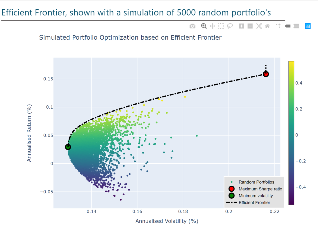
Visualising the Efficient Frontier
Now we create a function to create a plotly graph of the efficient frontier by calling our calculatedResults function above.
def EF_graph(meanReturns, covMatrix, riskFreeRate=0, constraintSet=(0,1)):
    """Return a graph ploting the min vol, max sr and efficient frontier"""
    maxSR_returns, maxSR_std, maxSR_allocation, minVol_returns, minVol_std, minVol_allocation, efficientList, targetReturns = calculatedResults(meanReturns, covMatrix, riskFreeRate, constraintSet)

    #Max SR
    MaxSharpeRatio = go.Scatter(
        name='Maximium Sharpe Ratio',
        mode='markers',
        x=[maxSR_std],
        y=[maxSR_returns],
        marker=dict(color='red',size=14,line=dict(width=3, color='black'))
    )

    #Min Vol
    MinVol = go.Scatter(
        name='Mininium Volatility',
        mode='markers',
        x=[minVol_std],
        y=[minVol_returns],
        marker=dict(color='green',size=14,line=dict(width=3, color='black'))
    )

    #Efficient Frontier
    EF_curve = go.Scatter(
        name='Efficient Frontier',
        mode='lines',
        x=[round(ef_std*100, 2) for ef_std in efficientList],
        y=[round(target*100, 2) for target in targetReturns],
        line=dict(color='black', width=4, dash='dashdot')
    )

    data = [MaxSharpeRatio, MinVol, EF_curve]

    layout = go.Layout(
        title = 'Portfolio Optimisation with the Efficient Frontier',
        yaxis = dict(title='Annualised Return (%)'),
        xaxis = dict(title='Annualised Volatility (%)'),
        showlegend = True,
        legend = dict(
            x = 0.75, y = 0, traceorder='normal',
            bgcolor='#E2E2E2',
            bordercolor='black',
            borderwidth=2),
        width=800,
        height=600)

    fig = go.Figure(data=data, layout=layout)
    return fig.show()