
In this tutorial we try to understand the difference between simple returns and log returns. We also talk about normality of financial data!
If we want to model returns using the normal distribution!
- SIMPLE RETURNS: The product of normally distributed variables is NOT normally distributed
- LOG RETURNS: The sum of normally distributed variables DOES follow a normal distribution
Also the log distribution bounds our stock price at 0. Which is a nice property to have and is consistent with reality.
Step 1: Import dependencies
import datetime as dt
import pandas as pd
import numpy as np
import pylab
import seaborn as sns
import scipy.stats as stats
from pandas_datareader import data as pdr
import plotly.offline as pyo

pyo.init_notebook_mode(connected=True)
pd.options.plotting.backend = 'plotly'
Step 2: get stock market data
Choose a date range and select stock to chart.
end = dt.datetime.now()
start = dt.datetime(2018,1,1)

df = pdr.get_data_yahoo('CBA.AX', start, end)
df.head()
Simple vs Log Returns
Firstly one period simple returns
\(R_t = \frac{P_t – P_{t-1}}{P_{t-1}} = \frac{P_t}{P_{t-1}} – 1\)
\(1 + R_t = \frac{P_t}{P_{t-1}}\)
Calculate Daily Simple Returns
simple_returns = df.Close.pct_change().dropna()
simple_returns
For multi-period k returns
\(1 + R_t(k) = \frac{P_t}{P_{t-1}}\frac{P_{t-1}}{P_{t-2}}…\frac{P_{t-k+1}}{P_{t-k}} = \frac{P_t}{P_{t-k}}\)
\(1 + R_t(k) = (1 + R_t)(1 + R_{t-1})…(1 + R_{t-k+1})\)
\(1 + R_t(k) = \prod_{i=0}^{k-1} (1 + R_{t-i})\)
Plot financial data and look at first and last share prices
df.Close.plot().update_layout(autosize=False,width=500,height=300).show(renderer="colab")
print('First', df.Close[0], 'Last', df.Close[-1])
Use simple returns & attempt to compute final price from starting price over time horizon
simple_returns.mean()
df.Close[0]*(1+simple_returns.mean())**len(simple_returns)
df.Close[0]*np.prod([(1+Rt) for Rt in simple_returns])
Log Returns
Now onto one period log returns:
\(r_t = \ln(1+R_t)\)
K-period log returns:
\(r_t(k) = \ln(1+R_t(k)) = \ln[(1+R_t)(1+R_{t-1})…(1+R_{t-k+1})]\)
\(r_t(k) = \ln(1+R_t(k)) = \ln(1+R_t) + \ln(1+R_{t-1}) + … + \ln(1+R_{t-k+1})\)
\(r_t(k) = \ln(1+R_t(k)) = r_t + r_{t-1} + … + r_{t-k+1} = \ln(P_t) – \ln(P_{t-k})\)
Compute log returns in python
log_returns = np.log(df.Close / df.Close.shift(1)).dropna()
log_returns

log_returns.mean()
df.Close[0] * np.exp(len(log_returns) * log_returns.mean())
AGAIN, THE MAIN REASON!
If we want to model returns using the normal distribution!
– SIMPLE RETURNS: The product of normally distribution variables is NOT normally distributed
– LOG RETURNS: The sum of normally distributed variables follows a normal distribution
Also the log distribution bounds our stock price at 0. Which is a nice property to have and is consistent with reality.
Histogram of log returns
log_returns.plot(kind='hist').update_layout(autosize=False,width=500,height=300).show(renderer="colab")
Is normality a good assumption for financial data?
The assumption that prices or more accurately log returns are normally distributed?
log_returns_sorted = log_returns.tolist()
log_returns_sorted.sort()
worst = log_returns_sorted[0]
best = log_returns_sorted[-1]

std_worst = (worst - log_returns.mean())/log_returns.std()
std_best = (best - log_returns.mean())/log_returns.std()
print('Assuming price is normally distributed: ')
print(' Standard dev. worst %.2f and best %.2f' %(std_worst, std_best))
print(' Probability of worst %.13f and best %.13f' %(stats.norm(0, 1).pdf(std_worst), stats.norm(0, 1).pdf(std_best)))
Testing for Normality
https://towardsdatascience.com/normality-tests-in-python-31e04aa4f411
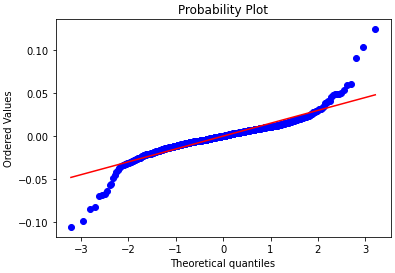
Q-Q or Quantile-Quantile Plots
It plots two sets of quantiles against one another i.e. theoretical quantiles against the actual quantiles of the variable.
stats.probplot(log_returns, dist='norm', plot=pylab)
print('Q-Q Plot')
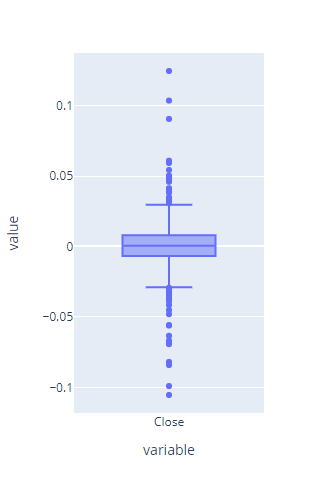
Box Plots
Box Plot also know as a box and whisker plot is another way to visualize the normality of a variable. It displays the distribution of data based on a five-number summary i.e. minimum, first quartile (Q1), median (Q2), third quartile (Q3) and maximum.
log_returns.plot(kind = 'box').update_layout(autosize=False,width=350,height=500).show(renderer="colab")
Hypothesis Testing / Statistical Inference ?
Why would you do it? – it can give a more objective answer!
Kolmogorov Smirnov test
The Kolmogorov Smirnov test computes the distances between the empirical distribution and the theoretical distribution and defines the test statistic as the supremum of the set of those distances.
The Test Statistic of the KS Test is the Kolmogorov Smirnov Statistic, which follows a Kolmogorov distribution if the null hypothesis is true. If the observed data perfectly follow a normal distribution, the value of the KS statistic will be 0. The P-Value is used to decide whether the difference is large enough to reject the null hypothesis:
The advantage of this is that the same approach can be used for comparing any distribution, not necessary the normal distribution only.
- Do not forget to assign arguments mean and standard deviation! (this was reminded by a subscriber – thanks)
ks_statistic, p_value = stats.kstest(log_returns, 'norm', args = (log_returns.mean(), log_returns.std()))
print(ks_statistic, p_value)
if p_value > 0.05:
    print('Probably Gaussian')
else:
    print('Probably not Gaussian')
Shapiro Wilk test
The Shapiro Wilk test is the most powerful test when testing for a normal distribution. It has been developed specifically for the normal distribution and it cannot be used for testing against other distributions like for example the KS test.
sw_stat, p = stats.shapiro(log_returns)
print('stat=%.3f, p=%.3f' % (sw_stat, p))
if p_value > 0.05:
    print('Probably Gaussian')
else:
    print('Probably not Gaussian')