
The Feynman–Kac analysis enables us to define a risk neutral probability in which we can price options. Let \(f_\mathbb{Q}(S_T)\) denote the terminal risk neutral (\(\mathbb{Q}\)-measure) probability at time \(T\) , and let \(F_\mathbb{Q}(S_T)\) denote the cumulative probability. A European call option at time \(t\), expiring at \(T\) , with strike price \(K\), is priced (\(\tau = T – t\)):
\(\large C(K, \tau) = \large E_\mathbb{Q}[e^{-r\tau} (S_T – K)^+]\)
\(\large C(K, \tau) = e^{-r\tau} \int^\infty_K (S_T – K)f_\mathbb{Q}(S_T)dS_T\)
In the case where \(f_\mathbb{Q}\) is the log-normal density and volatility is constant with respect to \(K\), this yields the Black–Scholes formula.
Under basic no-arbitrage restrictions, we can consider more general densities than the log-normal for the underlying. Breeden and Litzenberger (1978) show that the first derivative is a function of the cumulative distribution.
\(\large \frac{\delta C}{\delta K}|{K=S_T} = -e^{-r\tau}(1 – F\mathbb{Q}(S_T))\)
The second derivative then extracts the density
\(\large \frac{\delta^2 C}{\delta K^2}|{K=S_T} = e^{-r\tau}f \mathbb{Q}(S_T)\)
References:
Bruce Mizrach, Chapter 35: Estimating Implied Probabilities from Option Prices and the Underlying
http://econweb.rutgers.edu/mizrach/pubs/%5B42%5D-2010_Handbook.pdf
https://www.repository.utl.pt/bitstream/10400.5/3372/1/Tese_andre_novo_4.0.pdf
import numpy as np
import scipy as sc
import pandas as pd
from scipy import stats
import matplotlib.pyplot as plt
European Call Option with Stochastic Volatility
Risk-Neutral Dynamics:
Underlying process:
\(\large dS_{t} = r S_{t} dt + \sqrt{v_{t}} S_{t} dW^\mathbb{Q}_{s,t}\)
Variance process:
\(\large dv_{t} = \kappa (\theta – v_{t})dt + \sigma \sqrt{v_{t}} dW^\mathbb{Q}_{v,t}\)
- \(dW^\mathbb{Q}{S,t}\) Brownian motion of asset price
- \(dW^\mathbb{Q}{v,t}\) Brownian motion of asset’s price variance
- \(\rho^\mathbb{Q}\) correlation between \(dW^\mathbb{Q}{S,t}\) and \(dW^\mathbb{Q}{v,t}\)
# Initialise parameters
S0 = 100.0     # initial stock price
K = 150.0      # strike price
tau = 1.0        # time to maturity in years
r = 0.06       # annual risk-free rate

# Heston dependent parameters
kappa = 3              # rate of mean reversion of variance under risk-neutral dynamics
theta = 0.20**2        # long-term mean of variance under risk-neutral dynamics
v0 = 0.20**2           # initial variance under risk-neutral dynamics
rho = 0.98              # correlation between returns and variances under risk-neutral dynamics
sigma = 0.2            # volatility of volatility
lambd = 0              # risk premium of variance

2*kappa*theta, ' > ',sigma**2
Breeden-Litzenberger Formula
Let’s determine the risk-neutral probability distribution function (pdf), \(f _\mathbb{Q}\).
\(\large f _\mathbb{Q}(K, \tau) = e^{r \tau} \frac{\delta^2C(K,\tau)}{\delta K^2}\)
Use 2nd order finite difference approximation:
\(\large f_\mathbb{Q}(K, \tau) \approx e^{r\tau} \frac{C(K+\Delta_K,\tau) – 2C(K,\tau) + C(K-\Delta_K,\tau)}{(\Delta_K)^2}\)
Heston Model Characteristic Equation:
\(\large C(S_0, K, v_0, \tau) = \frac{1}{2}(S_0 – Ke^{-r \tau}) + \frac{1}{\pi} \int^\inf_0 \Re [ e^{r\tau} \frac{\varphi(\phi-i)}{i\phi K^{i\phi}} – K\frac{\varphi(\phi)}{i\phi K^{i\phi}} ] d\phi\)
\(\varphi(X_0, K, v_0,\tau; \phi) = e^{r \phi i \tau} S^{i \phi}[\frac{1-ge^{d\tau}}{1-g}]^{\frac{-2a}{\sigma^2}} exp[\frac{a \tau}{\sigma^2} (b_2 -\rho\sigma \phi i + d) + \frac{v_0}{\sigma^2}(b_2 -\rho\sigma \phi i + d)[\frac{1-e^{d\tau}}{1-ge^{d\tau}}]]\)
where:
\(d = \sqrt{(\rho\sigma \phi i – b)^2 + \sigma^2 (\phi i + \phi^2)}\)
\(g = \frac{b -\rho\sigma \phi i + d}{b -\rho\sigma \phi i – d}\)
\(a = \kappa \theta\)
\(b = \kappa + \lambda\)
https://www.maths.univ-evry.fr/pages_perso/crepey/Finance/051111_mikh%20heston.pdf
http://web.math.ku.dk/~rolf/teaching/ctff03/Gatheral.1.pdf
def heston_charfunc(phi, S0, v0, kappa, theta, sigma, rho, lambd, tau, r):

    # constants
    a = kappa*theta
    b = kappa+lambd

    # common terms w.r.t phi
    rspi = rho*sigma*phi*1j

    # define d parameter given phi and b
    d = np.sqrt( (rspi - b)**2 + (phi*1j+phi**2)*sigma**2 )

    # define g parameter given phi, b and d
    g = (b-rspi+d)/(b-rspi-d)

    # calculate characteristic function by components
    exp1 = np.exp(r*phi*1j*tau)
    term2 = S0**(phi*1j) * ( (1-g*np.exp(d*tau))/(1-g) )**(-2*a/sigma**2)
    exp2 = np.exp(a*tau*(b-rspi+d)/sigma**2 + v0*(b-rspi+d)*( (1-np.exp(d*tau))/(1-g*np.exp(d*tau)) )/sigma**2)

    return exp1*term2*exp2

def heston_price_rec(S0, K, v0, kappa, theta, sigma, rho, lambd, tau, r):
    args = (S0, v0, kappa, theta, sigma, rho, lambd, tau, r)

    P, umax, N = 0, 100, 650
    dphi=umax/N #dphi is width
    for j in range(1,N):
        # rectangular integration
        phi = dphi * (2*j + 1)/2 # midpoint to calculate height
        numerator = heston_charfunc(phi-1j,*args) - K * heston_charfunc(phi,*args)
        denominator = 1j*phi*K**(1j*phi)

        P += dphi * numerator/denominator

    return np.real((S0 - K*np.exp(-r*tau))/2 + P/np.pi)


strikes = np.arange(60, 180, 1.0)
option_prices = heston_price_rec(S0, strikes, v0, kappa, theta, sigma, rho, lambd, tau, r)

option_prices
Use 2nd order finite difference approximation:
\(\large f_\mathbb{Q}(K, \tau) \approx e^{r\tau} \frac{C(K+\Delta_K,\tau) – 2C(K,\tau) + C(K-\Delta_K,\tau)}{(\Delta_K)^2}\)
prices = pd.DataFrame([strikes, option_prices]).transpose()
prices.columns = ['strike', 'price']
prices['curvature'] = (-2 * prices['price'] +
prices['price'].shift(1) +
prices['price'].shift(-1)) / 1**2
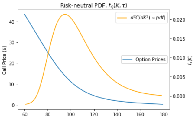
# And plotting...
fig = plt.figure()
ax = fig.add_subplot(111)
plt.ylabel('Call Price ($)')
ax2 = ax.twinx()
ax.plot(strikes, option_prices, label='Option Prices')
ax2.plot(prices['strike'], prices['curvature'], label='$d^2C/dK^2 (\sim pdf)$', color='orange')
ax.legend(loc="center right")
ax2.legend(loc="upper right")
plt.xlabel('Strikes (K)')
plt.ylabel('$f_\\tau(K)$')
plt.title('Risk-neutral PDF, $f_\mathbb{Q}(K, \\tau)$')
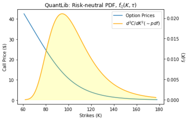
Let’s compare with QuantLib Heston Model
References:
Stack Exchange Question, Computing the Probability Density Function (PDF) for the Heston model
https://quant.stackexchange.com/questions/57827/computing-the-probability-density-function-pdf-for-the-heston-model
import QuantLib as ql
today = ql.Date(28, 5, 2022)
expiry_date = today + ql.Period(int(365*tau), ql.Days)

# Setting up discount curve
risk_free_curve = ql.FlatForward(today, r, ql.Actual365Fixed())
flat_curve = ql.FlatForward(today, 0.0, ql.Actual365Fixed())
riskfree_ts = ql.YieldTermStructureHandle(risk_free_curve)
dividend_ts = ql.YieldTermStructureHandle(flat_curve)

# Setting up a Heston model
heston_process = ql.HestonProcess(riskfree_ts, dividend_ts, ql.QuoteHandle(ql.SimpleQuote(S0)), v0, kappa, theta, sigma, rho)
heston_model = ql.HestonModel(heston_process)
heston_handle = ql.HestonModelHandle(heston_model)
heston_vol_surface = ql.HestonBlackVolSurface(heston_handle)

# Now doing some pricing and curvature calculations
vols = [heston_vol_surface.blackVol(tau, x) for x in strikes]

option_prices1 = []
for strike in strikes:
    option = ql.EuropeanOption( ql.PlainVanillaPayoff(ql.Option.Call, strike), ql.EuropeanExercise(expiry_date))

    heston_engine = ql.AnalyticHestonEngine(heston_model)
    option.setPricingEngine(heston_engine)

    option_prices1.append(option.NPV())

prices = pd.DataFrame([strikes, option_prices, option_prices1]).transpose()
prices.columns = ['strike', 'Rectangular Int','QuantLib']
prices['curvature'] = (-2 * prices['QuantLib'] + prices['QuantLib'].shift(1) + prices['QuantLib'].shift(-1)) / 1**2

# And plotting...
fig = plt.figure(figsize=(10,6))
ax = fig.add_subplot(111)
plt.ylabel('Call Price ($)')
plt.xlabel('Strikes (K)')
ax2 = ax.twinx()
lns1 = ax.plot(strikes, option_prices1, label='Option Prices')
lns2 = ax2.plot(prices['strike'], prices['curvature'], label='$d^2C/dK^2 (\sim pdf)$', color='orange')
ax2.fill_between(prices['strike'], prices['curvature'], color='yellow', alpha=0.2)

# added these three lines
lns = lns1+lns2
labs = [l.get_label() for l in lns]
ax.legend(lns, labs, loc=0)

# ax.legend(loc="center right")
# ax2.legend(loc="upper right")
plt.ylabel('$f_\\tau(K)$')
plt.title('QuantLib: Risk-neutral PDF, $f_\mathbb{Q}(K, \\tau)$')
What are the differences? – and why
The differences are mainly a result of the method of complex integration over very small increments.
Python has issues with round off errors at small values approximated by binary floating-point numbers.
https://stackoverflow.com/questions/15930381/python-round-off-error
https://docs.python.org/3/tutorial/floatingpoint.html
mse = np.mean( (option_prices - option_prices1)**2 )
print("QuantLib vs. Our Rect Int \n   Mean Squared Error: ", mse)
prices.dropna()
prices.head(40)
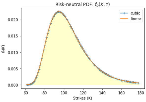
Interpolation of the Risk-Neutral density function
inter = prices.dropna()
pdf = sc.interpolate.interp1d(inter.strike, np.exp(r*tau)*inter.curvature, kind = 'linear')
pdfc = sc.interpolate.interp1d(inter.strike, np.exp(r*tau)*inter.curvature, kind = 'cubic')

strikes = np.arange(61, 179, 1.0)

plt.plot(strikes, pdfc(strikes), '-+', label='cubic')
plt.plot(strikes, pdf(strikes), label='linear')
plt.fill_between(strikes, pdf(strikes), color='yellow', alpha=0.2)
plt.xlabel('Strikes (K)')
plt.ylabel('$f_\\tau(K)$')
plt.title('Risk-neutral PDF: $f_\mathbb{Q}(K, \\tau)$')
plt.legend()
plt.show()
Cumulative distribution function
cdf = sc.interpolate.interp1d(inter.strike, np.cumsum(pdf(strikes)), kind = 'linear')

plt.plot(strikes, cdf(strikes))

plt.xlabel('Strikes (K)')
plt.ylabel('$F_\\tau(K)$')
plt.title('Risk-neutral CDF: $F_\mathbb{Q}(K, \\tau)$')
Using the Risk-neutral PDF to price ‘complex’ derivatives
Remember the RND function \(f^{\tau}_\mathbb{Q}(S_T)\) is defined at a particular time to expiry \(\tau\)
Call
\(\large C(K, \tau) = e^{-r\tau} \int^\infty_K (S_T – K)f^{\tau}_\mathbb{Q}(S_T)dS_T\)
Put
\(\large P(K, \tau) = e^{-r\tau} \int^K_{-\infty} (K – S_T)f^{\tau}_\mathbb{Q}(S_T)dS_T\)
http://econweb.rutgers.edu/mizrach/pubs/%5B42%5D-2010_Handbook.pdf
def integrand_call(x, K):
        return (x-K)*pdf(x)

def integrand_put(x, K):
        return (K-x)*pdf(x)

calls, puts = [], []
for K in strikes:
    # integral from K to infinity (looking at CDF, 179 last defined value on range)
    call_int, err = sc.integrate.quad(integrand_call, K, 178, limit=1000, args=K)

    # integral from -infinity to K (looking at CDF, 61 lowest defined value on range)
    put_int, err = sc.integrate.quad(integrand_put, 61, K, limit=1000, args=K)

    call = np.exp(-r*tau)*call_int
    calls.append( call )

    put = np.exp(-r*tau)*put_int
    puts.append( put )


rnd_prices = pd.DataFrame([strikes, calls, puts]).transpose()
rnd_prices.columns = ['strike', 'Calls','Puts']
rnd_prices.tail()