
# Import dependencies
import time
import math
import numpy as np
import pandas as pd
import datetime
import scipy as sc
import matplotlib.pyplot as plt
from pandas_datareader import data as pdr
from IPython.display import display, Latex
from statsmodels.graphics.tsaplots import plot_acf
# import data
def get_data(stocks, start, end):
    df = pdr.get_data_yahoo(stocks, start, end)
    return df

endDate = datetime.datetime.now()
startDate = endDate - datetime.timedelta(days=7000)

stock_prices = get_data('^GSPC', startDate, endDate)
print(startDate)
stock_prices.head()
Volatility clustering in financial time series
Paper: Volatility Clustering in Financial Markets:Empirical Facts and Agent–Based Models, Rama Cont. 2005.
The study of statistical properties of financial time series:
– Excess volatility
– Heavy Tails
– Volatilty clustering
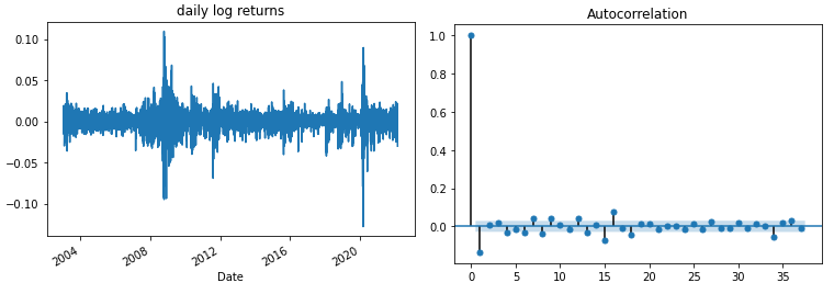
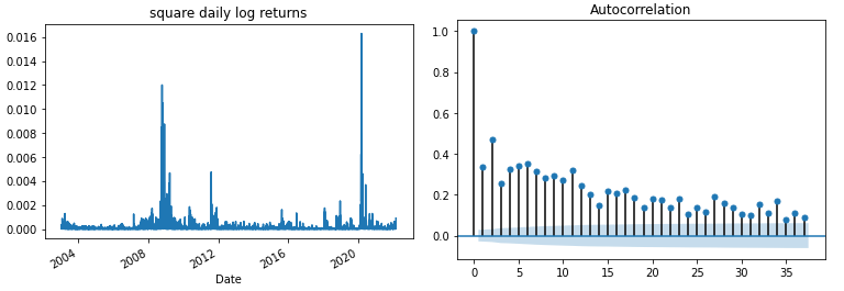
As noted by Mandelbrot [1], “large changes tend to be followed by large changes, of either sign, and small changes tend to be followed by small changes.” A quantitative manifestation of this fact is that, while returns themselves are uncorrelated, absolute returns \(|r_t|\) or their squares display a positive, significant and slowly decaying autocorrelation function: \(corr(|r_t|, |r_t+\tau|) > 0\) for \(\tau\) ranging from a few minutes to a several weeks.
[1] B. B. Mandelbrot (1963) The variation of certain speculative prices, Journal of Business, XXXVI (1963), pp. 392–417.
Denote by \(S_t\) the price of a financial asset and \(X_t = ln S_t\) its logarithm. Given a time scale \(\Delta\), the logreturn at scale \(\Delta\) is defined as:
\(r_t = X_{t+\Delta} – X_t = ln(S_t+\Delta S_t)\)
log_returns = np.log(stock_prices.Close/stock_prices.Close.shift(1)).dropna()
log_returns.plot()
plt.title('daily log returns')
plot_acf(log_returns)
plt.show()
log_returns_sq = np.square(log_returns)
log_returns_sq.plot()
plt.title('square daily log returns')
plot_acf(log_returns_sq)
plt.show()
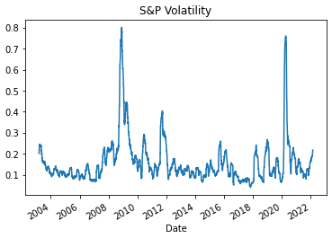
TRADING_DAYS = 40
volatility = log_returns.rolling(window=TRADING_DAYS).std()*np.sqrt(252)
volatility = volatility.dropna()
volatility.plot()
plt.title('S&P Volatility')
plt.show()
Ornstein-Uhlenbeck
Ornstein-Uhlenbeck is a stochastic process that is a stationary Gauss-Markov process.
\({\displaystyle dX_{t}=-\kappa \,X_{t}\,dt+\sigma \,dW_{t}}\)
Sometimes, an additional drift term is sometimes added – this is known as the Vasicek model:
\({\displaystyle dX_{t}=\kappa (\theta -X_{t})\,dt+\sigma \,dW_{t}}\)
Maximum Log-likelihood Estimation (MLE)
Probability Density Function of Normal Distribution is:
\(\Large f_\theta (x)=\frac{1}{\sqrt{2\pi \sigma^2}} e^{\frac{-(x-\mu)^2}{2 \sigma^2}}\) If we have random samples \(y_i, i = 1,…,N\) from a density \(f_\theta (y)\) indexed bu some parameter \(\theta\).
Joint Probability Density Function or Likelihood function:\( f(x_1,…x_n|\theta) = f(x_1|\theta)…f(x_n|\theta) = \prod^n_{i=1}f(X_i|\theta) = L(\theta)\)
The likelihood function is the density function regarded as a function of \(\theta\).\( L(\theta|x) = f(x|\theta), \theta \in \Theta\)
The maximum likelihood estimator (MLE):
\(\hat{\theta}(x) = arg \underset{\theta}{max} L(\theta|x)\)
Log-probability of the observed sample is:
\(l(\theta) = \sum^N_{i=1} log f_\theta (y_i)\)
The principle of maximum likelihood assumes that the most reasonable values for \(\theta\) are those for which the probability of the observed sample islargest.
Essentially we are completing least squares for the additive error model \(Y = f_\theta(X) + \epsilon\), with \(\epsilon \sim N(0, \sigma^2)\), is equivalent to maximum likelihood using the conditional likelihood:
\(f(Y|X, \theta) = N(log f_\theta (X), \sigma^2)\)
If we take the likelihood function and derive the partial dericatives with respect the each respective parameter, make equal to zero, then we solve for MLE.
\(L(\mu, \sigma^2 | \theta) = (\frac{1}{\sqrt{2\pi \sigma^2}} e^{\frac{-(x_1-\mu)^2}{2 \sigma^2}}) … \frac{1}{\sqrt{2\pi \sigma^2}} e^{\frac{-(x_n-\mu)^2}{2 \sigma^2}} = \frac{1}{\sqrt{(2\pi \sigma^2)^n}} e^{-\frac{1}{2\sigma^2}\sum^n_{i=1}(x_i-\mu)^2}\)
Log-likelihood function
\(l(\mu, \sigma^2 | \theta) = ln L(\mu, \sigma^2 | \theta) = -\frac{n}{2}(ln2\pi+ln\sigma^2)-\frac{1}{2\sigma^2}\sum^n_{i=1}(x_i-\mu)^2\)
Sometimes this is not differentiable but in the case of the normal distribution we can use Lagrange multiplier method to find maximisation parameters.
– \(\frac{\delta}{\delta \mu}ln L(\mu, \sigma^2 | \theta) = 0 = \frac{1}{\sigma^2}\sum^n_{i=1}(x_i-\mu) = \frac{1}{\sigma^2}n(\overline{x} – \mu)\)- \(\hat{\mu}(x) = \overline{x}\)
This is a local maximum because the second partial derivative with respect to \(\mu\) is negative, hence concave function.
– \(\frac{\delta}{\delta \sigma^2}ln L(\mu, \sigma^2 | \theta) = 0 = -\frac{n}{2\sigma^2}+\frac{1}{2(\sigma^2)^2}\sum^n_{i=1}(x_i-\mu)^2 = -\frac{n}{2(\sigma^2)^2}(\sigma^2+\frac{1}{n}\sum^n_{i=1}(x_i-\mu)^2)\)- \(\hat{\sigma}^2(x)=\frac{1}{n}\sum^n_{i=1}(x_i-\overline{x})^2\)
def MLE_norm(x):
    mu_hat = np.mean(x)
    sigma2_hat = np.var(x)
    return mu_hat, sigma2_hat

mu = 5
sigma = 2.5
N = 10000

np.random.seed(0)
x = np.random.normal(loc=mu, scale=sigma, size=(N,))

mu_hat, sigma2_hat = MLE_norm(x)

for_mu_hat = '$\hat{\mu} = '+format(round(mu_hat,2))+'$'
for_sigma2_hat = '$\hat{\sigma} = '+format(round(np.sqrt(sigma2_hat),2))+'$'

print('The MLE for data is:')
display(Latex(for_mu_hat))
display(Latex(for_sigma2_hat))
Performing MLE numerically
If the log likelihood function wasn’t continuous or differentiable. Can solve numerically through an optimisation problem where objective function is …
The maximum likelihood estimator (MLE):\(\hat{\theta}(x) = arg\) \(\underset{\theta}{max}\) \(L(\theta|x)\)
\(\hat{\theta}(x) = arg\) \(\underset{\theta}{max}\) \(ln\) \(L(\theta|x)\)
\(L(\theta) = \prod^n_{i=1}f(X_i|\theta)\)
\(ln f(X∣\theta)=\sum_{i=1}^N ln f(x_i∣\theta)\)
def log_likelihood(theta, x):
    mu = theta[0]
    sigma = theta[1]

    l_theta = np.sum( np.log( sc.stats.norm.pdf(x, loc=mu, scale=sigma) ) )

    return -l_theta

def sigma_pos(theta):
    sigma = theta[1]
    return sigma

cons_set = {'type':'ineq', 'fun': sigma_pos}

theta0 = [2,3]
opt = sc.optimize.minimize(fun=log_likelihood, x0=theta0, args=(x,), constraints=cons_set)

for_mu_hat = '$\hat{\mu} = '+format(round(opt.x[0],2))+'$'
for_sigma2_hat = '$\hat{\sigma} = '+format(round(opt.x[1],2))+'$'

print('The MLE for data is:')
display(Latex(for_mu_hat))
display(Latex(for_sigma2_hat))
So what’s the distribution function of Ornstein-Uhlenbeck process?
Solution use, Ito Calculus to find equation for \(d(X_t)\) and then determine Expectation and Variance of \(X_t\).
Find dynamics of \(X_t\)
1. Rearrange
– \({\displaystyle dX_{t}=\kappa (\theta -X_{t})\,dt+\sigma \,dW_{t}}\)- \(dX_t= \kappa \theta dt -\kappa X_t dt+\sigma dW_t\)- \(dX_t + \kappa X_t dt = \kappa \theta dt + \sigma dW_t\)
We recognise: \(d(e^{\kappa t} X_t) = e^{\kappa t}dX_t + \kappa e^{\kappa t} X_t dt\),
2. so multiply equation through by \(e^{\kappa t}\) term. Take integral over time horizon \(t \in [0,T]\)
– \(\int^T_0 d(e^{\kappa t} X_t) = \int^T_0 \kappa \theta e^{\kappa t} dt + \int^T_0 \sigma e^{\kappa t} dW_t\)- \( e^{\kappa T} X_T – X_0 = \kappa \theta \frac{e^{\kappa T}-1}{\kappa} + \sigma \int^T_0 e^{\kappa t} dW_t\)- \( X_T = X_0 e^{-\kappa T} + \theta (1 – e^{-\kappa T}) + \sigma \int^T_0 e^{-\kappa (T-t)} dW_t\)
Find \(E[X_T]\)
– \(E[X_T] = E[X_0 e^{-\kappa T} + \theta (1 – e^{-\kappa T}) + \sigma \int^T_0 e^{-\kappa (T-t)} dW_t]\)- \(E[X_T] = X_0 e^{-\kappa T} + \theta (1 – e^{-\kappa T})\)
Find \(Var[X_T] = E[(X_T- E[X_T])^2]\). Substitute in \(X_T\) and \(E[X_T]\) derived above.- \(Var[X_T] = E[(\sigma \int^T_0 e^{-\kappa (T-t)} dW_t)^2]\)
– Remember Ito Lemma, only term left after cross multiply \(dWdW = dt\). – \(Var[X_T] = \sigma^2 \int^T_0 e^{-2\kappa (T-t)} dt\)- \(Var[X_T] = \sigma^2 \frac{1-e^{-2\kappa T}}{2 \kappa}\)- \(Var[X_T] = \frac{\sigma^2}{2 \kappa}(1-e^{-2\kappa T}) \)
Now the stochastic process is normally distributed with \(E[X_t]\) and \(Var[X_t]\).- \(X_t \sim N(\mu, \sigma)\)- \(X_t = \mu + \sigma Z_t\) where \(Z_t \sim N(0, 1)\)
– \(X_{t+\Delta t} = X_t e^{-\kappa T} + \theta (1 – e^{-\kappa T}) + \sigma \sqrt{\frac{(1-e^{-2\kappa T})}{2 \kappa}} N(0,1)\)
MLE of Ornstein-Uhlenbeck process
– \(X_t \sim N(\mu, \overline{\sigma})\)
– \(E[X_{t+\delta t}] = X_t e^{-\kappa \delta t} + \theta (1 – e^{-\kappa \delta t})\)- \(Var[X_{t+\delta t}] = \frac{\sigma^2}{2 \kappa}(1-e^{-2\kappa \delta t}) \)
\(\Large f_\overline{\theta} (x_{t+\delta t} | x_t, \kappa, \theta, \sigma)=\frac{1}{\sqrt{2\pi \overline{\sigma}^2}} e^{\frac{-(x-\mu)^2}{2 \overline{\sigma}^2}}\)
– \(\mu(x_t, \kappa, \theta) = x_t e^{-\kappa \delta t} + \theta (1 – e^{-\kappa \delta t})\)
– \(\overline{\sigma}(\kappa, \sigma) = \sigma \sqrt{\frac{(1-e^{-2\kappa \delta t})}{2 \kappa}}\)
def mu(x, dt, kappa, theta):
    ekt = np.exp(-kappa*dt)
    return x*ekt + theta*(1-ekt)

def std(dt, kappa, sigma):
    e2kt = np.exp(-2*kappa*dt)
    return sigma*np.sqrt((1-e2kt)/(2*kappa))

def log_likelihood_OU(theta_hat, x):
    kappa = theta_hat[0]
    theta = theta_hat[1]
    sigma = theta_hat[2]

    x_dt = x[1:]
    x_t = x[:-1]

    dt = 1/252

    mu_OU = mu(x_t, dt, kappa, theta)
    sigma_OU = std(dt, kappa, sigma)

    l_theta_hat = np.sum( np.log( sc.stats.norm.pdf(x_dt, loc=mu_OU, scale=sigma_OU) ) )

    return -l_theta_hat

def kappa_pos(theta_hat):
    kappa = theta_hat[0]
    return kappa

def sigma_pos(theta_hat):
    sigma = theta_hat[2]
    return sigma

vol = np.array(volatility)

cons_set = [{'type':'ineq', 'fun': kappa_pos},
            {'type':'ineq', 'fun': sigma_pos}]

theta0 = [1,3,1]
opt = sc.optimize.minimize(fun=log_likelihood_OU, x0=theta0, args=(vol,), constraints=cons_set)

kappa = round(opt.x[0],3)
theta = round(opt.x[1],3)
sigma = round(opt.x[2],3)
vol0 = vol[-1]

for_kappa_hat = '$\hat{\kappa} = '+str(kappa)+'$'
for_theta_hat = '$\hat{\Theta} = '+str(theta)+'$'
for_sigma_hat = '$\hat{\sigma} = '+str(sigma)+'$'

print('The MLE for data is:')
display(Latex(for_kappa_hat))
display(Latex(for_theta_hat))
display(Latex(for_sigma_hat))
print('Last Volatility', round(vol0,3))
Simulating Ornstein-Uhlenbeck process:
\({\displaystyle dX_{t}=\kappa (\theta -X_{t})\,dt+\sigma \,dW_{t}}\)
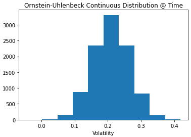
Continuous-time stochastic process:
\( X_t = X_0 e^{-\kappa t} + \theta (1 – e^{-\kappa t}) + \sigma \int^t_0 e^{-\kappa (t-s)} dW_s\)
# define parameters
Time = 0.3
M = 10000

Z = np.random.normal(size=(M))

def mu(x, dt, kappa, theta):
    ekt = np.exp(-kappa*dt)
    return x*ekt + theta*(1-ekt)

def std(dt, kappa, sigma):
    e2kt = np.exp(-2*kappa*dt)
    return sigma*np.sqrt((1-e2kt)/(2*kappa))

drift_OU = mu(vol0, Time, kappa, theta)
diffusion_OU = std(Time, kappa, sigma)
vol_OU = drift_OU + diffusion_OU*Z

plt.hist(vol_OU)
plt.title('Ornstein-Uhlenbeck Continuous Distribution @ Time')
plt.xlabel('Volatility')
plt.show()
Discretised SDE
Euler-Maryuama discretisation: This is an approximation of variance…
\(\Delta x_{t+1} = \kappa(\theta – x_t) \Delta t + \sigma \sqrt{\Delta t} \epsilon_t\)
where parameters are assigned as from above optimisation
# Initialise Parameters for discretization
days = 1
years = 2

dt = days/252

M = 1000
N = int(years/dt)
Recursive Function
vol_OU = np.full(shape=(N, M), fill_value=vol0)
Z = np.random.normal(size=(N, M))

def OU_recursive(t, vol_OU):
    # Return the final state
    if t == N:
        return vol_OU

    # Thread the state through the recursive call
    else:
        drift_OU = kappa*(theta - vol_OU[t-1])*dt
        diffusion_OU = sigma*np.sqrt(dt)
        vol_OU[t] = vol_OU[t-1] + drift_OU + diffusion_OU*Z[t]
        return OU_recursive(t + 1, vol_OU)


start_time = time.time()
vol_OU = OU_recursive(0, vol_OU)
print('Execution time', time.time() - start_time)
vol_OU = np.concatenate( (np.full(shape=(1, M), fill_value=vol0), vol_OU ) )
plt.plot(vol_OU)
plt.title('Ornstein-Uhlenbeck Euler Discretization')
plt.ylabel('Volatility')
plt.show()
Python Loop
vol_OU = np.full(shape=(N, M), fill_value=vol0)
Z = np.random.normal(size=(N, M))

start_time = time.time()
for t in range(1,N):
    drift_OU = kappa*(theta - vol_OU[t-1])*dt
    diffusion_OU = sigma*np.sqrt(dt)
    vol_OU[t] = vol_OU[t-1] + drift_OU + diffusion_OU*Z[t]
print('Execution time', time.time() - start_time)

vol_OU = np.concatenate( (np.full(shape=(1, M), fill_value=vol0), vol_OU ) )
plt.plot(vol_OU)
plt.title('Ornstein-Uhlenbeck Euler Discretization')
plt.ylabel('Volatility')
plt.show()
Not sure why recursive function is so slow in google colab – suspect that there is no benefit here of using RAM for in-memory storage vs actual computer compiling?? Comment in Discord channel if you know why?