1993: Stochastic volatility model by Heston
The Heston model is a useful model for simulating stochastic volatility and its effect on the potential paths an asset can take over the life of an option.
- Popular because of easy closed-form solution for European option pricing
- no risk of negative variances
- incorporation of leverage effect
This allows for more effective modeling than the Black-Scholes formula allows due to its restrictive assumption of constant volatility.
Heston Model SDE
The heston model is defined by a system of SDEs, to describe the movement of asset prices, where anasset’s price and volatility follow random, Brownian motion processes (this is under real world measure \(\mathbb{P}\)):
\(\large dS_t = \mu S_t dt + \sqrt{v_t}S_t dW^\mathbb{P}_{S,t}\)
\(\large dv_t = \kappa(\theta – v_t)dt +\sigma \sqrt{v_t} dW^\mathbb{P}_{v,t}\)
Where the variables are:
– \(\sigma\) volatility of volatility
– \(\theta\) long-term price variance
– \(\kappa\) rate of reversion to the long term price variance
– \(dW^\mathbb{P}_{S,t}\) Brownian motion of asset price
– \(dW^\mathbb{P}_{v,t}\) Brownian motion of asset’s price variance
– \(\rho^\mathbb{P}\) correlation between \(dW^\mathbb{P}_{S,t}\) and \(dW^\mathbb{P}_{v,t}\)
Dynamics under risk-neutral measure \(\mathbb{Q}\):
\(\large dS_t = r S_t dt + \sqrt{v_t}S_t dW^\mathbb{Q}_{S,t}\)
\(\large dv_t = \kappa^\mathbb{Q}(\theta^\mathbb{Q} – v_t)dt +\sigma^\mathbb{Q} \sqrt{v_t} dW^\mathbb{Q}_{v,t}\)
Heston Model for Monte Carlo Simulations
Obviously as discussed one of the nice things about the Heston model for European option prices is that there is a closed-form solution once you have the characteristic function. So discretisation of the SDE is not required for valuing a European option, however if you would like to value other option types with complex features using the Heston model than you can use the following code:
Euler Discretisation of SDEs
Great resource for explanation here: Euler and Milstein Discretization by Fabrice Douglas Rouah https://frouah.com/finance%20notes/Euler%20and%20Milstein%20Discretization.pdf
\(\Large S_{i+1} = S_i e^{(r-\frac{v_i}{2}) \Delta t + \sqrt{v_{i}}\Delta tW^\mathbb{Q}_{S,i+1}}\)
\(\large v_{i+1} = v_i + \kappa(\theta – v_t)\Delta t +\sigma \sqrt{v_i} \Delta t W^\mathbb{Q}_{v,i+1}\)
Import dependencies
import numpy as np
import seaborn as sns
import matplotlib.pyplot as plt
from py_vollib_vectorized import vectorized_implied_volatility as implied_vol
Define Parameters
Here we just define the parameters of the model under risk-neutral dynamics, however in a following tutorial I will show how to calibrate Heston model parameters under risk-neutral dynamics to real option market prices.
# Parameters
# simulation dependent
S0 = 100.0             # asset price
T = 1.0                # time in years
r = 0.02               # risk-free rate
N = 252                # number of time steps in simulation
M = 1000               # number of simulations

# Heston dependent parameters
kappa = 3              # rate of mean reversion of variance under risk-neutral dynamics
theta = 0.20**2        # long-term mean of variance under risk-neutral dynamics
v0 = 0.25**2           # initial variance under risk-neutral dynamics
rho = 0.7              # correlation between returns and variances under risk-neutral dynamics
sigma = 0.6            # volatility of volatility

theta, v0
Monte Carlo Simulation
Because we have a recursive function, we have to step through time within our simulation. However we can simulate the Brownian motions of the asset and variances outside of the for loop.
def heston_model_sim(S0, v0, rho, kappa, theta, sigma,T, N, M):
    """
    Inputs:
     - S0, v0: initial parameters for asset and variance
     - rho   : correlation between asset returns and variance
     - kappa : rate of mean reversion in variance process
     - theta : long-term mean of variance process
     - sigma : vol of vol / volatility of variance process
     - T     : time of simulation
     - N     : number of time steps
     - M     : number of scenarios / simulations

    Outputs:
    - asset prices over time (numpy array)
    - variance over time (numpy array)
    """
    # initialise other parameters
    dt = T/N
    mu = np.array([0,0])
    cov = np.array([[1,rho],
                    [rho,1]])

    # arrays for storing prices and variances
    S = np.full(shape=(N+1,M), fill_value=S0)
    v = np.full(shape=(N+1,M), fill_value=v0)

    # sampling correlated brownian motions under risk-neutral measure
    Z = np.random.multivariate_normal(mu, cov, (N,M))

    for i in range(1,N+1):
        S[i] = S[i-1] * np.exp( (r - 0.5*v[i-1])*dt + np.sqrt(v[i-1] * dt) * Z[i-1,:,0] )
        v[i] = np.maximum(v[i-1] + kappa*(theta-v[i-1])*dt + sigma*np.sqrt(v[i-1]*dt)*Z[i-1,:,1],0)

    return S, v
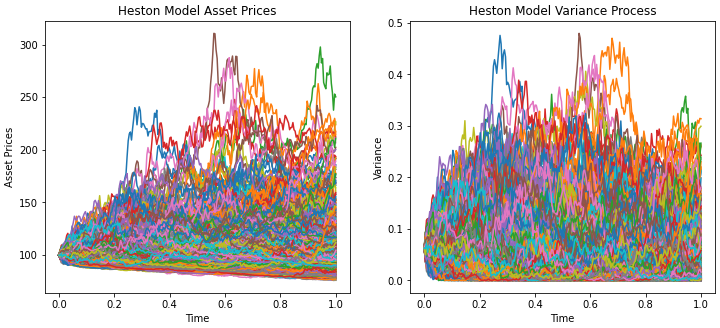
rho_p = 0.98
rho_n = -0.98

S_p,v_p = heston_model_sim(S0, v0, rho_p, kappa, theta, sigma,T, N, M)
S_n,v_n = heston_model_sim(S0, v0, rho_n, kappa, theta, sigma,T, N, M)
Plotting the asset prices and variance over time
fig, (ax1, ax2)  = plt.subplots(1, 2, figsize=(12,5))
time = np.linspace(0,T,N+1)
ax1.plot(time,S_p)
ax1.set_title('Heston Model Asset Prices')
ax1.set_xlabel('Time')
ax1.set_ylabel('Asset Prices')

ax2.plot(time,v_p)
ax2.set_title('Heston Model Variance Process')
ax2.set_xlabel('Time')
ax2.set_ylabel('Variance')

plt.show()
Asset price distribution with different correlations
# simulate gbm process at time T
gbm = S0*np.exp( (r - theta**2/2)*T + np.sqrt(theta)*np.sqrt(T)*np.random.normal(0,1,M) )

fig, ax = plt.subplots()

ax = sns.kdeplot(S_p[-1], label=r"$\rho= 0.98$", ax=ax)
ax = sns.kdeplot(S_n[-1], label=r"$\rho= -0.98$", ax=ax)
ax = sns.kdeplot(gbm, label="GBM", ax=ax)

plt.title(r'Asset Price Density under Heston Model')
plt.xlim([20, 180])
plt.xlabel('$S_T$')
plt.ylabel('Density')
plt.legend()
plt.show()

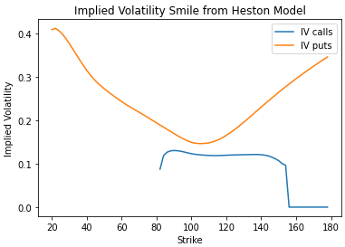
Capturing the Volatililty Smile in Option Pricing
rho = -0.7
S,v = heston_model_sim(S0, v0, rho, kappa, theta, sigma,T, N, M)

# Set strikes and complete MC option price for different strikes
K = np.arange(20,180,2)

puts = np.array([np.exp(-r*T)*np.mean(np.maximum(k-S,0)) for k in K])
calls = np.array([np.exp(-r*T)*np.mean(np.maximum(S-k,0)) for k in K])

put_ivs = implied_vol(puts, S0, K, T, r, flag='p', q=0, return_as='numpy', on_error='ignore')
call_ivs = implied_vol(calls, S0, K, T, r, flag='c', q=0, return_as='numpy')

plt.plot(K, call_ivs, label=r'IV calls')
plt.plot(K, put_ivs, label=r'IV puts')

plt.ylabel('Implied Volatility')
plt.xlabel('Strike')

plt.title('Implied Volatility Smile from Heston Model')
plt.legend()
plt.show()