import numpy as np
import scipy as sc
import pandas as pd
from scipy import stats
import matplotlib.pyplot as plt
Recall that for Pricing a European Call Option under Risk-Neutral Pricing
\(\large E_\mathbb{Q}[e^{-rT} (S_0e^{Z_T} – K)^+]\), where \(\large Z_T \sim N((r – \frac{\sigma^2}{2})T, \sigma^2T)\)
Of course, a European Call Option has a closed form solution – BS
def blackScholes(r, S, K, T, sigma, opt_type="c"):
    "Calculate BS price of call/put"
    d1 = (np.log(S/K) + (r + sigma**2/2)*T)/(sigma*np.sqrt(T))
    d2 = d1 - sigma*np.sqrt(T)
    try:
        if opt_type == "c":
            price = S*sc.stats.norm.cdf(d1, 0, 1) - K*np.exp(-r*T)*sc.stats.norm.cdf(d2, 0, 1)
        elif opt_type == "p":
            price = K*np.exp(-r*T)*sc.stats.norm.cdf(-d2, 0, 1) - S*sc.stats.norm.cdf(-d1, 0, 1)
        return price
    except:
        print("Please confirm option type, either 'c' for Call or 'p' for Put!")

# Initialise parameters
S0 = 100.0     # initial stock price
K = 170.0      # strike price
T = 1.0        # time to maturity in years
r = 0.06       # annual risk-free rate
vol = 0.20     # volatility (%)

dt = T
nudt = (r - 0.5*vol**2)*dt
nudt2 = (np.log(K/S0)-0.5*vol**2)*dt
volsdt = vol*np.sqrt(dt)

BS = blackScholes(r, S0, K, T, vol)
print("Black Scholes Price: ", round(BS,4))
Benefits of Importance Sampling?
\(\large E[f(x)] = \int f(x)p(x) dx \approx \frac{1}{n}\sum_i f(x_i)\)
Example: Just How Unlucky is a 25 Standard Deviation Loss?
http://www.columbia.edu/~mh2078/MonteCarlo/MCS_AdvVarRed_MasterSlides.pdf
\(\large \theta = P(X \geq 25) = E[I_{X\geq 25}]\) when \(\large X \sim N(0,1)\)
M = 1000000
Z = np.random.normal(0,1, M)

# Indicator function, count number of sampled variables above 25
ZT = np.where(Z>25,1,0)
X = np.mean( ZT )

# Calculate standard error and 95% Condifence intervals
sigma = np.std(ZT)
SE = sigma/np.sqrt(M)
CIs = [X-SE*1.96,X+SE*1.96]

print('95% Confidence Levels for 25 St Dev. Returns are [{:0.3e}, {:0.3e}]'.format(CIs[0], CIs[1]))
Method of Importance Sampling – change of distribution
\(\large E[f(x)] = \int f(x)p(x) dx = \int f(x)\frac{p(x)}{q(x)}q(x) dx \approx \frac{1}{n}\sum_i f(x_i)\frac{p(x)}{q(x)}\)
For the Normal Distribution (and many other distributions), we can work out an analytical form for the distribution PDF ratio p(x)/q(x).
\(\large \theta = E[I_{X\geq 25}] = \int^\infty_{-\infty} I_{X\geq 25} \frac{1}{\sqrt{2 \pi}} e^{-\frac{x^2}{2}}dx\)
\(\large = \int^\infty_{-\infty} I_{X\geq 25} \left( \frac{\frac{1}{\sqrt{2 \pi}} e^{-\frac{x^2}{2}}}{\frac{1}{\sqrt{2 \pi}} e^{-\frac{{x-\mu}^2}{2}}} \right) {\frac{1}{\sqrt{2 \pi}} e^{-\frac{{x-\mu}^2}{2}}}dx\)
\(\large = \int^\infty_{-\infty} I_{X\geq 25} e^{-\mu X + \frac{\mu^2}{2}}dx\)
M = 1000
mu=25

Z = np.random.normal(mu,1, M)

# Method 1 - use scipy stats PDF functions
p = sc.stats.norm(0, 1)
q = sc.stats.norm(mu, 1)

ZT = np.where(Z>25,1,0)*p.pdf(Z)/q.pdf(Z)

# Method 2 - direct with analytical ratio
ZT = np.where(Z>25,1,0)*np.exp(-mu*Z + mu**2/2)

X = np.mean( ZT )
sigma = np.std(ZT)
SE = sigma/np.sqrt(M)
CIs = [X-SE*1.96,X+SE*1.96]

print('95% Confidence Levels for 25 St Dev. Returns are [{:0.3e}, {:0.3e}]'.format(CIs[0], CIs[1]))
Importance Sampling and Radon-Nikodym derivative
Importance Sampling: \(\large E[f(x)] = \int f(x)p(x) dx = \int f(x)\frac{p(x)}{q(x)}q(x) dx \approx \frac{1}{n}\sum_i f(x_i)\frac{p(x)}{q(x)}\)
Radon-Nikodym derivative: \(\large E_\mathbb{Q}[f(S_T)] = E_{\mathbb{Q}_{0}}[f(S_T) \frac{\mathbb{dQ}}{\mathbb{dQ}_{0}}]\)
There exists a change of measure called the Radon-Nikodym derivative: \(\Large \frac{\mathbb{dQ}}{\mathbb{dQ}_{0}}\)
So conduct a simulation under a new measure \(\Large \mathbb{Q}_{0}\) and then multiply by the ratio of the two probability density functions, or the Radon Nikodym derivative of one process with respect to the other.
Note: For more complicated processes and derivatives one need to use the densities given by Girsanovs Theorem within the monte carlo simulation.
https://sas.uwaterloo.ca/~dlmcleis/s906/chapt5.pdf
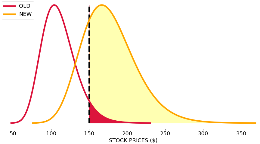
Using a Far OTM Put Option to demonstrate the power of Importance Sampling
\(\large E_\mathbb{Q}[e^{-rT} (S_0e^{Z_T} – K)^+]\), where \(\large Z_T \sim N((r – \frac{\sigma^2}{2})T, \sigma^2T)\)
\(\large E_\mathbb{Q_0}[e^{-rT} (S_0e^{Z_T} – K)^+]\), where \(\large Z_T \sim N((log(K/S_0) – \frac{\sigma^2}{2})T, \sigma^2T)\)\
M = 100
N = 52
#precompute constants
dt = T/N
nudt = (r - 0.5*vol**2)*dt
nudt2 = (np.log(K/S0)-0.5*vol**2)*dt
volsdt = vol*np.sqrt(dt)
lnS = np.log(S0)
# Monte Carlo Method
Z = np.random.normal(0,1,size=(N, M))
delta_lnSt = nudt + volsdt*Z
lnSt = lnS + np.cumsum(delta_lnSt, axis=0)
lnSt = np.concatenate( (np.full(shape=(1, M), fill_value=lnS), lnSt ) )
delta_lnSt2 = nudt2 + volsdt*Z
lnSt2 = lnS + np.cumsum(delta_lnSt2, axis=0)
lnSt2 = np.concatenate( (np.full(shape=(1, M), fill_value=lnS), lnSt2 ) )
ST = np.exp(lnSt)
ST2 = np.exp(lnSt2)
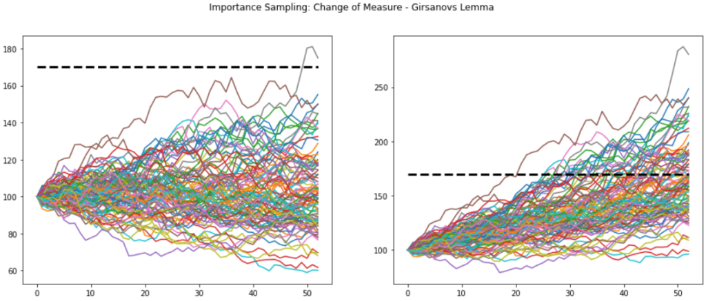
fig, (ax1, ax2) = plt.subplots(1, 2, figsize=(16,6))
fig.suptitle('Importance Sampling: Change of Measure - Girsanovs Lemma')
ax1.plot(ST)
ax1.plot([0,N],[K,K],'k--',linewidth=3)
ax2.plot(ST2)
ax2.plot([0,N],[K,K],'k--',linewidth=3)
plt.show()
# Initialise parameters
S0 = 100.0     # initial stock price
K = 170.0      # strike price
T = 1.0        # time to maturity in years
r = 0.06       # annual risk-free rate
vol = 0.20     # volatility (%)

dt = T
nudt = (r - 0.5*vol**2)*dt
nudt2 = (np.log(K/S0)-0.5*vol**2)*dt
volsdt = vol*np.sqrt(dt)

nudt, nudt2
Choosing the correct distribution to minimize variance
\(\large E[f(x)] = \int f(x)p(x) dx = \int f(x)\frac{p(x)}{q(x)}q(x) dx \approx \frac{1}{n}\sum_i f(x_i)\frac{p(x)}{q(x)}\)
\(\large E_\mathbb{Q}[f(S_T)] = E_{\mathbb{Q}_{0}}[f(S_T) \frac{\mathbb{dQ}}{\mathbb{dQ}_{0}}]\)
Unfortunately there is no general way to final the optimal \(q(x)\) distribution under \(\mathbb{dQ}_{0}\) distribution. But we can find the relatively optimal g to reduce variance.
\(\Large min_\mu E_p \left[ f^2(x) \frac{p(x)}{q_\mu(x)} \right]\)
References:
Variance Reduction Techniques of Importance Sampling Monte Carlo Methods for Pricing Options
Journal of Mathematical Finance, 2013, 3, 431-436
Published Online November 2013 (http://www.scirp.org/journal/jmf)
http://dx.doi.org/10.4236/jmf.2013.34045
p = sc.stats.norm(nudt,volsdt)
q = lambda mu: sc.stats.norm(mu, volsdt)
z_T = lambda x, mu, sig: mu + sig*x
f_0 = lambda z: np.exp(-r*T)*np.maximum(0, S0*np.exp(z)-K)
M = 1000000
def arg_min(x):
x_T = np.random.normal(0, 1, M)
z = z_T(x_T,nudt,volsdt)
return np.mean( f_0(z)**2 * p.pdf(z)/q(x).pdf(z) )
mu_star = sc.optimize.fmin(lambda x: arg_min(x), nudt2, disp=True)
mu_star
C0_is, SE_is = [], []
for M in np.arange(100,1000+100,100):
mu = mu_star[0]
x = np.random.randn(M)
z = z_T(x,mu,volsdt)
CT = f_0(z) * p.pdf(z)/q(mu).pdf(z)
C0 = np.mean( CT )
sigma = np.sqrt( np.sum( (CT - C0)**2) / (M-1) )
SE = sigma/np.sqrt(M)
C0_is.append(C0)
SE_is.append(SE)
C0_is = np.array(C0_is)
SE_is = np.array(SE_is)
print("Call value is ${0} with SE +/- {1}".format(np.round(C0_is,3),np.round(SE_is,3)))
C0_wo, SE_wo = [], []
for M in np.arange(100,1000+100,100):
x = np.random.randn(M)
z = z_T(x, nudt, volsdt)
CT = f_0(z)
C0 = np.mean( CT )
sigma = np.sqrt( np.sum( (CT - C0)**2) / (M-1) )
SE = sigma/np.sqrt(M)
C0_wo.append(C0)
SE_wo.append(SE)
C0_wo = np.array(C0_wo)
SE_wo = np.array(SE_wo)
print("Call value is ${0} with SE +/- {1}".format(np.round(C0_wo,3),np.round(SE_wo,3)))
SE_Ratio = SE_wo/SE_is
print("Standard Error Reduction Factor {0}".format(np.round(SE_Ratio,3)))
import pandas as pd
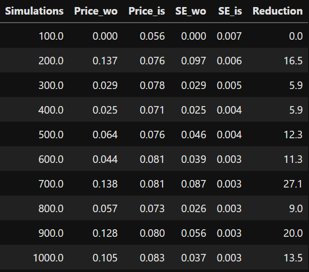
M = np.arange(100,1000+100,100)
prices = pd.DataFrame(np.array([M, C0_wo.round(3), C0_is.round(3), SE_wo.round(3), SE_is.round(3), SE_Ratio.round(1)]).T,
columns=['Simulations','Price_wo', 'Price_is','SE_wo', 'SE_is', 'Reduction'])
print("Black Scholes Price: ", round(BS,4))
prices