
In this tutorial we will investigate ways we can reduce the variance of results from a Monte Carlo simulation method when valuing financial derivatives. The mathematic notation and examples are from Les Clewlow and Chris Strickland’s book Implementing Derivatives Models.
Unfortunately, although a great method for approximating option values with complex payoffs or high dimensionality, in order to get an acceptably accurate estimate we must perform a large number of simulations M. Instead we can lean on Variance Reduction methods which work on the same principles as that of hedging an option position. i.e. the variability of a hedged option portfolio will have a smaller variance that that of it’s unhedged counterpart.
# Import dependencies
import math
import numpy as np
import pandas as pd
import datetime
import scipy.stats as stats
import matplotlib.pyplot as plt
Antithetic Variates
Let’s write an option on asset \(S_1\) and another option on asset \(S_2\) that is perfectly negatively correlated with \(S_1\) and which currently has the same price. \(S_1\) and \(S_2\) satisfy the following Stochastic Differential Equations:
\(\large dS_{1,t} = rdS_{1,t}dt+\sigma dS_{1,t}dz_t\)
\(\large dS_{2,t} = rdS_{2,t}dt-\sigma dS_{2,t}dz_t\)
Since the price and volatility of the two assets are identical, so is the value of these two options. However, the variance of a portfolio pay-off containing both of these contracts is much less than the variance of the pay-off of each individual contract. In essence we are removing the large spike in probability distribution of a single contract pay-off. i.e. Basic Intuition: when one option pays out, the other does not.
Implementation of Antithetic Variate
To implement an antithetic variate we create a hypothetical asset which is perfectly negatively correlated with the original asset. Implementation is very simple, and if we consider the example of the European Call Option (as in last weeks video). Our simulated pay-offs are under the following \(S_t\) dynamics:
\(\large S_{t+\Delta t} = S_{t} \exp( \nu \Delta t + \sigma (z_{t+\Delta t}- z_t) )\)
Where \((z_{t+\Delta t}- z_t) \sim N(0,\Delta t) \sim \sqrt{\Delta t} N(0,1) \sim \sqrt{\Delta t} \epsilon_i\)
Contract Simulation
– \(\large C_{T,i} = max(0, S \exp( \nu \Delta T + \sigma \sqrt{T} (\epsilon_i) ) – K)\)
– \(\large \bar{C}_{T,i} = max(0, S \exp( \nu \Delta T + \sigma \sqrt{T} (-\epsilon_i) ) – K)\)
# initial derivative parameters
S = 101.15          #stock price
K = 98.01           #strike price
vol = 0.0991        #volatility (%)
r = 0.015            #risk-free rate (%)
N = 10              #number of time steps
M = 1000            #number of simulations

market_value = 3.86 #market price of option
T = ((datetime.date(2022,3,17)-datetime.date(2022,1,17)).days+1)/365    #time in years
print(T)
Slow Solution – Steps
We break it down into slow discretized steps, although for the purposes of a European Call Option we do not have to take steps as the discretization perfectly represents the SDE.
# Precompute constants
dt = T/N
nudt = (r - 0.5*vol**2)*dt
volsdt = vol*np.sqrt(dt)
lnS = np.log(S)

# Standard Error Placeholders
sum_CT = 0
sum_CT2 = 0

# Monte Carlo Method
for i in range(M):
    lnSt1 = lnS
    lnSt2 = lnS
    for j in range(N):
        # Perfectly Negatively Correlated Assets
        epsilon = np.random.normal()
        lnSt1 = lnSt1 + nudt + volsdt*epsilon
        lnSt2 = lnSt2 + nudt - volsdt*epsilon

    ST1 = np.exp(lnSt1)
    ST2 = np.exp(lnSt2)
    CT = 0.5 * ( max(0, ST1 - K) + max(0, ST2 - K) )
    sum_CT = sum_CT + CT
    sum_CT2 = sum_CT2 + CT*CT

# Compute Expectation and SE
C0 = np.exp(-r*T)*sum_CT/M
sigma = np.sqrt( (sum_CT2 - sum_CT*sum_CT/M)*np.exp(-2*r*T) / (M-1) )
SE = sigma/np.sqrt(M)

print("Call value is ${0} with SE +/- {1}".format(np.round(C0,2),np.round(SE,2)))
Fast Solution – Vectorized
- Only 1 Step is Necessary in this example!
For simple processes where the SDE does not need to be approximated like in the case of Geometric Brownian Motion used for calculating a European Option Price, we can just simulate the variables at the final Time Step as Brownian Motion scales with time and independent increments.
#precompute constants
N = 1
dt = T/N
nudt = (r - 0.5*vol**2)*dt
volsdt = vol*np.sqrt(dt)
lnS = np.log(S)

# Monte Carlo Method
Z = np.random.normal(size=(N, M))
delta_lnSt1 = nudt + volsdt*Z
delta_lnSt2 = nudt - volsdt*Z
lnSt1 = lnS + np.cumsum(delta_lnSt1, axis=0)
lnSt2 = lnS + np.cumsum(delta_lnSt2, axis=0)

# Compute Expectation and SE
ST1 = np.exp(lnSt1)
ST2 = np.exp(lnSt2)
CT = 0.5 * ( np.maximum(0, ST1[-1] - K) + np.maximum(0, ST2[-1] - K) )
C0 = np.exp(-r*T)*np.sum(CT)/M

sigma = np.sqrt( np.sum( (CT - C0)**2) / (M-1) )
SE = sigma/np.sqrt(M)

print("Call value is ${0} with SE +/- {1}".format(np.round(C0,2),np.round(SE,2)))
Compare without Antithetic Variate
#precompute constants
N = 1
dt = T/N
nudt = (r - 0.5*vol**2)*dt
volsdt = vol*np.sqrt(dt)
lnS = np.log(S)

# Monte Carlo Method
Z = np.random.normal(size=(N, M))
delta_lnSt = nudt + volsdt*Z
lnSt = lnS + np.cumsum(delta_lnSt, axis=0)
lnSt = np.concatenate( (np.full(shape=(1, M), fill_value=lnS), lnSt ) )

# Compute Expectation and SE
ST = np.exp(lnSt)
CT = np.maximum(0, ST - K)
C0w = np.exp(-r*T)*np.sum(CT[-1])/M

sigma = np.sqrt( np.sum( (CT[-1] - C0)**2) / (M-1) )
SEw = sigma/np.sqrt(M)

print("Call value is ${0} with SE +/- {1}".format(np.round(C0,2),np.round(SE,2)))
Visualisation of Convergence
x1 = np.linspace(C0-3*SE, C0-1*SE, 100)
x2 = np.linspace(C0-1*SE, C0+1*SE, 100)
x3 = np.linspace(C0+1*SE, C0+3*SE, 100)
xw = np.linspace(C0w-3*SEw, C0w+3*SEw, 100)

s1 = stats.norm.pdf(x1, C0, SE)
s2 = stats.norm.pdf(x2, C0, SE)
s3 = stats.norm.pdf(x3, C0, SE)
sw = stats.norm.pdf(xw, C0w, SEw)

plt.fill_between(x1, s1, color='tab:blue',label='> StDev')
plt.fill_between(x2, s2, color='cornflowerblue',label='1 StDev')
plt.fill_between(x3, s3, color='tab:blue')
plt.plot(xw, sw, 'g-')
plt.fill_between(xw, sw, alpha=0.2, color='tab:green', label='w/o Antithetic')

plt.plot([C0,C0],[0, max(s2)*1.1], 'k',
        label='Theoretical Value')
plt.plot([C0w,C0w],[0, max(s2)*1.1], color='tab:green',
        label='Value w/o Antithetic')
plt.plot([market_value,market_value],[0, max(s2)*1.1], 'r',
        label='Market Value')

plt.ylabel("Probability")
plt.xlabel("Option Price")
plt.legend()
plt.show()
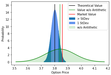
Benefits of Antithetic Variance Reduction
- By using pairs \((\epsilon_i, -\epsilon_i)\) in the simulation we can now achieve a more accurate estimate from M pairs of \((C_{T,i}, \bar{C}_{T,i})\) than from 2M of \({C}_{T,i}\) .
- It is also computationally cheaper to generate the pair \((C_{T,i}, \bar{C}_{T,i})\) than two instances of \(C_{T,i}\)
- Method also ensures that mean of the normally distributed samples \(\epsilon\) is exactly zero with helps improve the simulation