
Monte Carlo Pricing of European arithmetic Asian options
In this tutorial we will investigate the Monte Carlo simulation method for use in valuing financial derivatives. The mathematic notation and examples are from Les Clewlow and Chris Strickland’s book Implementing Derivatives Models.
Valuation of Financial Derivatives through Monte Carlo Simulations is only possible by using the Financial Mathematics of Risk-Neutral Pricing and simulating risk-neutral asset paths.
\(\begin{equation}\LARGE \frac{C_t}{B_t} = \mathbb{E}_{\mathbb{Q}}[\frac{C_T}{B_T}\mid F_t]\end{equation}\)
Note: This is the Risk-neutral Expectation Pricing Formula in Continuous Time
# Import dependencies
import time
import numpy as np
import pandas as pd
from scipy.stats import norm
from datetime import datetime
import matplotlib.pyplot as plt
Path-Dependent Options – Asian Options
In this example we are pricing a European arithmetic Asian call option. The option pays the difference between the arithmetic average of the asset price \(A_T\) and the strike price \(K\) at the maturity date \(T\). The arithmetic average is taken on a set of observations of the asset price \(S_{T_i}\) which we assume follows a GBM at dates \(t_i = 1,…,N\)
For an Asian (average price) option: \(A_T = \frac{1}{N}\sum^N_{i=1}S_{t_i}\)
Payoff at maturity date is : \(C_T[T_1,T_2] = f(S_T) = max(0, A_T – K)\)
\(\begin{equation}\large C(t,T_1, T_2) = e^{-r(T_2 – t)}\mathbb{E}_{\mathbb{Q}}[C_T[T_1,T_2] \mid F_t]\end{equation}\)
\(\begin{equation}\large C(t,T_1, T_2) = e^{-r(T_2 – t)}\mathbb{E}_{\mathbb{Q}}[(\frac{1}{T_2 – T_1} \int^{T_2}_{T_1} f(u,u)du – K)^+ \mid F_t]\end{equation}\)
Q1 2023 Electricity Average Rate Option
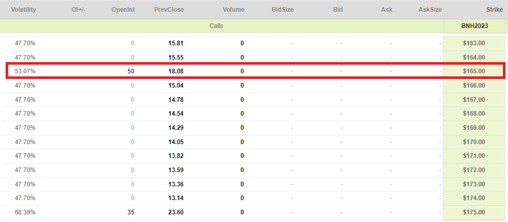
In the National Electricity Market (NEM), there are 5 seperate markets for each state. We will be valuing a Q1 2023 Electricity Asian Option in the NSW market, with:
- \(F0 = 135.89\)
- \(Strike = 165.00\)
- \(t = 22/4/2022\)
- \(T_1 = 1/1/2023\)
- \(T_2 = 31/3/2023\)
- \(T_2-T_1 = 90 days\)
Contract specification, average taken on 288 trading intervals each day over future contract period, Q1 90 day period. Hence we will have 25920 observations for our arithmetic average.
The Futures Contract Price for Q123

The Asian Call Option Price for Q123 at K = 165
t = datetime(2022,4,22)
T1 = datetime(2023,1,1)
T2 = datetime(2023,3,31)
Q123_days = ((T2 - T1).days+1)

# Initialise parameters
S0 = 135.89               # initial stock price
K = 165.00                # strike price
T = ((T2-t).days)/365     # time to maturity in years
r = 0.0                   # annual risk-free rate
vol = 0.5307              # volatility (%)

N = Q123_days*288         # number of time steps
M = 1000                  # number of simulations

Q123_days, N
In Reality!
Electricity Average Rate Options in Australia / NZ Energy Markets are settled against the final futures prices. As futures are settled against the arithmetic average of the wholesale energy market price. Therefore final futures price is the arithmetic average of wholesale electricity price.
Reference Price for Option Exercise In accordance with the final Settlement Price of the underlyingfutures contract as determined on the Third Business Day after theFinal Trading Day.
Method of Option Exercise On the Third Business Day after the Final Trading Day all in-themoney options are automatically exercised into the underlyingfutures contract and cash settled. Deny Automatic Exercise Requestsare not permitted. Exercise Requests for out-of-the-money optionsand/or at-the-money options are not permitted.
What that means?
These options can be priced using blackscholes until the end of the quarter.
def blackScholes(r, S, K, T, sigma, type="c"):
    "Calculate BS price of call/put"
    d1 = (np.log(S/K) + (r + sigma**2/2)*T)/(sigma*np.sqrt(T))
    d2 = d1 - sigma*np.sqrt(T)
    try:
        if type == "c":
            price = S*norm.cdf(d1, 0, 1) - K*np.exp(-r*T)*norm.cdf(d2, 0, 1)
        elif type == "p":
            price = K*np.exp(-r*T)*norm.cdf(-d2, 0, 1) - S*norm.cdf(-d1, 0, 1)
        return price
    except:
        print("Please confirm option type, either 'c' for Call or 'p' for Put!")

print("Black Scholes Option Price: ", round(blackScholes(r, S0, K, T, vol, "c"),2))
To demonstrate Pricing of an Average Rate Option
And to make things more interesting… let’s trade OTC, a bespoke Average Rate Option over Q123 with the underlying as the futures contract.
Let’s say that the average rate option prices are determined by the average of the (closing) daily futures prices across the Q123 period.
OTC (Bespoke) Arithmetic Average Options Price Q123 Futures Contract
Slow Solution Steps
# slow steps - discretized every day
N = Q123_days

T_tT2 = ((T2-t).days+1)/365
T_tT1 = (T1-t).days/365
print("Start averaging from T1", round(T_tT1,2), "to T2", round(T_tT2,2))

obs_times = np.linspace(T_tT1,T_tT2,N+1)
# Include starting time, uneven time delta's
obs_times[0]=0
dt = np.diff(obs_times)
print("Number of time steps:", len(dt))

start_time = time.time()

nudt = np.full(shape=(N), fill_value=0.0)
volsdt = np.full(shape=(N), fill_value=0.0)

# Precompute constants
for i in range(N):
    nudt[i] = (r - 0.5*vol**2)*dt[i]
    volsdt[i] = vol*np.sqrt(dt[i])

# Standard Error Placeholders
sum_CT = 0
sum_CT2 = 0

# Monte Carlo Method
for i in range(M):

    St = S0
    At_sum = 0

    for j in range(N):
        epsilon = np.random.normal()
        St = St*np.exp( nudt[j] + volsdt[j]*epsilon )
        At_sum += St

    A = At_sum/N
    CT = max(0, A - K)

    sum_CT = sum_CT + CT
    sum_CT2 = sum_CT2 + CT*CT

# Compute Expectation and SE
C0_slow = np.exp(-r*T)*sum_CT/M
sigma = np.sqrt( (sum_CT2 - sum_CT*sum_CT/M)*np.exp(-2*r*T) / (M-1) )
SE_slow = sigma/np.sqrt(M)

time_comp_slow = round(time.time() - start_time,4)
print("Call value is ${0} with SE +/- {1}".format(np.round(C0_slow,3),np.round(SE_slow,3)))
print("Computation time is: ", time_comp_slow)
Fast Implementation – Vectorized with Numpy
# fast steps - discretized every day (288 trading intervals)
N = Q123_days

obs_times = np.linspace(T_tT1,T_tT2,N+1)
# Include starting time, uneven time delta's
obs_times[0]=0
dt = np.diff(obs_times)
print("Number of time steps:", len(dt))

start_time = time.time()

nudt = np.full(shape=(N,M), fill_value=0.0)
volsdt = np.full(shape=(N,M), fill_value=0.0)

# Precompute constants
for i in range(N):
    nudt[i,:] = (r - 0.5*vol**2)*dt[i]
    volsdt[i,:] = vol*np.sqrt(dt[i])

# Monte Carlo Method
Z = np.random.normal(size=(N, M))
delta_St = nudt + volsdt*Z
ST = S0*np.cumprod( np.exp(delta_St), axis=0)
AT = np.cumsum(ST, axis=0)/N
ST = np.concatenate( (np.full(shape=(1, M), fill_value=S0), ST ) )

CT = np.maximum(0, AT[-1] - K)
C0_fast = np.exp(-r*T)*np.sum(CT)/M

sigma = np.sqrt( np.sum( (np.exp(-r*T)*CT - C0_fast)**2) / (M-1) )
sigma = np.std(np.exp(-r*T)*CT)
SE_fast = sigma/np.sqrt(M)

time_comp_fast = round(time.time() - start_time,4)
print("Call value is ${0} with SE +/- {1}".format(np.round(C0_fast,3),np.round(SE_fast,3)))
print("Computation time is: ", time_comp_fast)
MC Variance Reduction Comparison
Antithetic Variates
start_time = time.time()

nudt = np.full(shape=(N,M), fill_value=0.0)
volsdt = np.full(shape=(N,M), fill_value=0.0)

# Precompute constants
for i in range(N):
    nudt[i,:] = (r - 0.5*vol**2)*dt[i]
    volsdt[i,:] = vol*np.sqrt(dt[i])

# Monte Carlo Method
Z = np.random.normal(size=(N, M))
delta_St1 = nudt + volsdt*Z
delta_St2 = nudt - volsdt*Z
ST1 = S0*np.cumprod( np.exp(delta_St1), axis=0)
ST2 = S0*np.cumprod( np.exp(delta_St2), axis=0)
AT1 = np.cumsum(ST1, axis=0)/N
AT2 = np.cumsum(ST2, axis=0)/N
# ST = np.concatenate( (np.full(shape=(1, M), fill_value=S0), ST ) )

CT = 0.5 * ( np.maximum(0, AT1[-1] - K) + np.maximum(0, AT2[-1] - K) )
C0_av = np.exp(-r*T)*np.sum(CT)/M

sigma = np.sqrt( np.sum( (np.exp(-r*T)*CT - C0_av)**2) / (M-1) )
sigma = np.std(np.exp(-r*T)*CT)
SE_av = sigma/np.sqrt(M)

time_comp_av = round(time.time() - start_time,4)
print("Call value is ${0} with SE +/- {1}".format(np.round(C0_av,3),np.round(SE_av,3)))
print("Computation time is: ", time_comp_av)
Geometric Asian Option Control Variate
There is no analytical solution for an arithmetic Asian option, however there is for a geometric Asian option. This is because the geometric average is the product of lognormally distributed variables and therefore it is also lognormally distributed.
For an Geometric Asian (Geometric average price) option: \(G_T = (\prod^N_{i=1}S_{t_i})^{\frac{1}{N}}\)
Payoff at maturity date is : \(C_T[T_1,T_2] = f(S_T) = max(0, G_T – K)\)
Closed form solution: \(C_{geometric \ asian} = S_0 A_j N(d_{n-j} + \sigma \sqrt{T_{2,n-j}}) – Ke^{-rT}N(d_{n-j})\)
where:
\(d_{n-j} = \frac{ln(\frac{S_0}{K})+(r-\frac{\sigma^2}{2})T_{1,n-j}+ln(B_j)}{\sigma \sqrt{T_{2,n-j}}}\)
\(A_j = B_je^{-r(T-T_{1,n-j})-\sigma^2(T_{1,n-j}-T_{2,n-j})/2}\)
\(T_{1,n-j} = \frac{n-j}{n}(T – \frac{(n-j-1)h}{2})\)
\(T_{2,n-j} = (\frac{n-j}{n})^2 T – \frac{(n-j)(n-j-1)(4n-4j+1)}{6n^2}h\)
\(B_j = (\prod^n_{j=1} \frac{ST-(n-j)h}{S})^{1/n}\), \(B_0 = 1\)
n is the number of observations to form the average, h is the observation frequency, j is the numberof observations past in the averaging period
def discrete_geometric_asian(K, dt, S, vol, r, N):
    n, h, j = len(dt), dt[-1], 0
    T = np.cumsum(dt)[-1]
    T1nj = (T-(n-j-1)*h/2)*(n-j)/n
    T2nj = T*((n-j)/n)**2 - (n-j)*(n-j-1)*(4*n-4*j+1)*h/(6*n**2)
    Bj = (np.cumprod(np.array([(S*T - (n-j)*h)/S for j in range(1,n+1)]))[-1])**(1/n)
    Bj = 1 # no oberservations past
    Aj = Bj*np.exp(-r*(T-T1nj)-0.5*vol**2*(T2nj-T1nj))
    dnj = (np.log(S/K)+(r-0.5*vol**2)*T1nj + np.log(Bj))/(vol*np.sqrt(T2nj))
    C = S*Aj*norm.cdf(dnj + vol*np.sqrt(T2nj), 0, 1) - K*np.exp(-r*T)*norm.cdf(dnj)
    return C

discrete_geometric_asian(K, dt, S0, vol, r, N)
Simulate the difference between arithmetic and geometric Asian Options
The Geometric Asian option makes a good static hedge style control variate for the arithmetic option.
Instead of using the delta of the geometric asian option as a delta hedge control variate, we instead simulate a portfolio that is long the arithmetic and short the geometric asian option. This avoids the computation of calculating the delta at each time step and simulation path.
We then just add back the Analytical price of the Geometric Asian Option back to the MC portfolio simulation.
start_time = time.time()

nudt = np.full(shape=(N,M), fill_value=0.0)
volsdt = np.full(shape=(N,M), fill_value=0.0)

# Precompute constants
for i in range(N):
    nudt[i,:] = (r - 0.5*vol**2)*dt[i]
    volsdt[i,:] = vol*np.sqrt(dt[i])

# Monte Carlo Method
Z = np.random.normal(size=(N, M))
delta_St = nudt + volsdt*Z
ST = S0*np.cumprod( np.exp(delta_St), axis=0)
AT = np.cumsum(ST, axis=0)/N
GT = np.cumprod(ST**(1/N), axis=0)


CT = np.maximum(0, AT[-1] - K) - np.maximum(0, GT[-1] - K)

C0_cv = np.exp(-r*T)*np.sum(CT)/M

sigma = np.sqrt( np.sum( (np.exp(-r*T)*CT - C0_cv)**2) / (M-1) )
sigma = np.std(np.exp(-r*T)*CT)
SE_cv = sigma/np.sqrt(M)

C0_cv += discrete_geometric_asian(K, dt, S0, vol, r, N)

time_comp_cv = round(time.time() - start_time,4)
print("Call value is ${0} with SE +/- {1}".format(np.round(C0_cv,3),np.round(SE_cv,3)))
print("Computation time is: ", time_comp_cv)
Combined Antithetic and control Variate
start_time = time.time()

nudt = np.full(shape=(N,M), fill_value=0.0)
volsdt = np.full(shape=(N,M), fill_value=0.0)

# Precompute constants
for i in range(N):
    nudt[i,:] = (r - 0.5*vol**2)*dt[i]
    volsdt[i,:] = vol*np.sqrt(dt[i])

# Monte Carlo Method
Z = np.random.normal(size=(N, M))
delta_St1 = nudt + volsdt*Z
delta_St2 = nudt - volsdt*Z
ST1 = S0*np.cumprod( np.exp(delta_St1), axis=0)
ST2 = S0*np.cumprod( np.exp(delta_St2), axis=0)
AT1 = np.cumsum(ST1, axis=0)/N
AT2 = np.cumsum(ST2, axis=0)/N
GT1 = np.cumprod(ST1**(1/N), axis=0)
GT2 = np.cumprod(ST2**(1/N), axis=0)

CT = 0.5 * ( np.maximum(0, AT1[-1] - K) - np.maximum(0, GT1[-1] - K)
            + np.maximum(0, AT2[-1] - K) - np.maximum(0, GT2[-1] - K))


C0_acv = np.exp(-r*T)*np.sum(CT)/M

sigma = np.sqrt( np.sum( (np.exp(-r*T)*CT - C0_acv)**2) / (M-1) )
sigma = np.std(np.exp(-r*T)*CT)
SE_acv = sigma/np.sqrt(M)

C0_acv += discrete_geometric_asian(K, dt, S0, vol, r, N)

time_comp_acv = round(time.time() - start_time,4)
print("Call value is ${0} with SE +/- {1}".format(np.round(C0_acv,3),np.round(SE_acv,3)))
print("Computation time is: ", time_comp_acv)
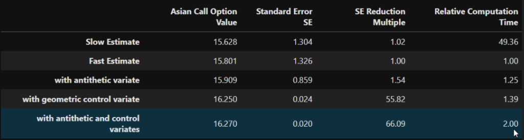
Comparing Variance Reduction Methods
C0_variates = [C0_slow, C0_fast, C0_av, C0_cv, C0_acv]
se_variates = [SE_slow, SE_fast, SE_av, SE_cv, SE_acv]
se_red = [round(SE_fast/se,2) for se in se_variates]
comp_time = [time_comp_slow, time_comp_fast, time_comp_av, time_comp_cv, time_comp_acv]
rel_time = [round(mc_time/time_comp_fast,2) for mc_time in comp_time]
data = {'Asian Call Option Value': np.round(C0_variates,3),
        'Standard Error SE': np.round(se_variates,3),
        'SE Reduction Multiple': se_red,
        'Relative Computation Time': rel_time}

# Creates pandas DataFrame.
df = pd.DataFrame(data, index =['Slow Estimate', 'Fast Estimate', 'with antithetic variate',
'with geometric control variate', 'with antithetic and control variates'])
df
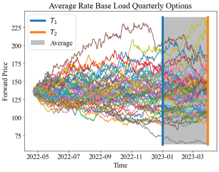
Visualisation
T_tot = (T2-t).days/365
T_start = (T1-t).days/365
M = 50
N = (T2-t).days

# precompute constants
dt = T/N
nudt = (r - 0.5*vol**2)*dt
volsdt = vol*np.sqrt(dt)

# Monte Carlo Method
Z = np.random.normal(size=(N, M))
delta_St = nudt + volsdt*Z
ST = S0*np.cumprod( np.exp(delta_St), axis=0)
ST = np.concatenate( (np.full(shape=(1, M), fill_value=S0), ST ) )
from matplotlib.patches import Rectangle
import matplotlib.dates as mdates

fig, ax = plt.subplots(figsize=(8,6))

plt.rcParams["font.family"] = "Times New Roman"
plt.rcParams["font.size"] = "16"

tx = pd.date_range(start=t,end=T2)
ax.plot(tx,ST)
ax.plot([T1, T1],[np.amin(ST),np.amax(ST)], linewidth=5, label='$T_1$')
ax.plot([T2, T2],[np.amin(ST),np.amax(ST)], linewidth=5, label='$T_2$')

# convert to matplotlib date representation
start = mdates.date2num(T1)+1
end = mdates.date2num(T2)-1
width = end - start

ax.add_patch(Rectangle((start,np.amin(ST)),width,np.amax(ST)-np.amin(ST),
                       alpha=0.5,
                    facecolor='grey',
                    lw=4, label='Average'))
plt.xlabel('Time')
plt.ylabel('Forward Price')
plt.title('Average Rate Base Load Quarterly Options')

plt.legend()
plt.show()