Pricing an Up-and-Out Barrier Option

In this tutorial we will investigate the Monte Carlo simulation method for use in valuing financial derivatives. The mathematic notation and examples are from Les Clewlow and Chris Strickland’s book Implementing Derivatives Models.

Valuation of Financial Derivatives through Monte Carlo Simulations is only possible by using the Financial Mathematics of Risk-Neutral Pricing and simulating risk-neutral asset paths.

\(\begin{equation}\LARGE \frac{C_t}{B_t} = \mathbb{E}_{\mathbb{Q}}[\frac{C_T}{B_T}\mid F_t]\end{equation}\)

Note: This is the Risk-neutral Expectation Pricing Formula in Continuous Time

# Import dependencies
import time
import numpy as np
import matplotlib.pyplot as plt

Geometric Brownian Motion Dynamics

Here we have constant interest rate so the discount factor is \(\exp(-rT)\), and the stock dynamics are modelled with Geometric Brownian Motion (GBM).
\(\large dS_t = rS_tdt+\sigma S_tdW_t\)
In terms of the stock price S, we have the following solution under risk-neutral dynamics:
\(\large S_{t+\Delta t} = S_{t} \exp( \nu \Delta t + \sigma \sqrt{\Delta t} \epsilon_i )\)
Where, \(\nu = r – \frac{1}{2} \sigma ^ 2\)

Key Differences for Path-Dependent Options

In pricing complex or exotic path dependent options, a popular product is the barrier option. These are standard European option expiration style options, however the options cease to exist or only comes into existence if the underlying price crosses a pretermined barrier level.

This barrier level can have either continuous or discrete barrier monitoring \(\large \tau\).
For an up-and-out barrier put option: \(C_T = f(S_T) = (K-S_T)^{+}Ind{(\max \limits_{t \in \tau} S_t < H)}\)
In other words for all simulations \(m \in M\):
– if \(t \in \tau\) and \(S_t \geq H\) then \(C_T = 0 \)
– else if \(t \notin \tau\) or \(S_t < H\) then \(C_T = (K-S_T)^{+}\)

# Initialise parameters
S0 = 100      # initial stock price
K = 100       # strike price
T = 1         # time to maturity in years
H = 125       # up-and-out barrier price/value
r = 0.01      # annual risk-free rate
vol = 0.2     # volatility (%)

N = 100       # number of time steps
M = 1000      # number of simulations

Slow Solution – Steps

Here we simulate stock price \(S_t\) directly because we require this value during the calculation to compare to the barrier \(H\).

start_time = time.time()

# Precompute constants
dt = T/N
nudt = (r - 0.5*vol**2)*dt
volsdt = vol*np.sqrt(dt)
erdt = np.exp(r*dt)

# Standard Error Placeholders
sum_CT = 0
sum_CT2 = 0

# Monte Carlo Method
for i in range(M):
    
    # Barrier Crossed Flag
    BARRIER = False
    St = S0
    
    for j in range(N):
        epsilon = np.random.normal()
        Stn = St*np.exp( nudt + volsdt*epsilon )
        St = Stn
        if St >= H:
            BARRIER = True
            break
            
    if BARRIER:
        CT = 0
    else:
        CT = max(0, K - St)
        
    sum_CT = sum_CT + CT
    sum_CT2 = sum_CT2 + CT*CT

# Compute Expectation and SE
C0 = np.exp(-r*T)*sum_CT/M
sigma = np.sqrt( (sum_CT2 - sum_CT*sum_CT/M)*np.exp(-2*r*T) / (M-1) )
SE = sigma/np.sqrt(M)

print("Call value is ${0} with SE +/- {1}".format(np.round(C0,2),np.round(SE,3)))
print("Computation time is: ", round(time.time() - start_time,4))

Fast Implementation – Vectorized with Numpy

np.any() is a function that returns True when ndarray passed to the first parameter contains at least one True element, and returns False otherwise

start_time = time.time()

#precompute constants
dt = T/N
nudt = (r - 0.5*vol**2)*dt
volsdt = vol*np.sqrt(dt)
erdt = np.exp(r*dt)

# Monte Carlo Method
Z = np.random.normal(size=(N, M)) 
delta_St = nudt + volsdt*Z
ST = S0*np.cumprod( np.exp(delta_St), axis=0)
ST = np.concatenate( (np.full(shape=(1, M), fill_value=S0), ST ) )

# Copy numpy array for plotting
S = np.copy(ST)

# Apply Barrier Condition to ST numpy array
mask = np.any(ST >= H, axis=0)
ST[:,mask] = 0

CT = np.maximum(0, K - ST[-1][ST[-1] != 0])
C0 = np.exp(-r*T)*np.sum(CT)/M

sigma = np.sqrt( np.sum( (np.exp(-r*T)*CT - C0)**2) / (M-1) )
sigma = np.std(np.exp(-r*T)*CT)
SE = sigma/np.sqrt(M)

print("Call value is ${0} with SE +/- {1}".format(np.round(C0,2),np.round(SE,3)))
print("Computation time is: ", round(time.time() - start_time,4))

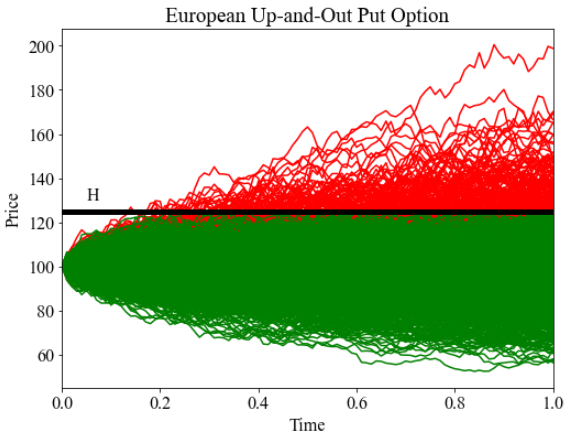
Visualisation

plt.figure(figsize=(8,6))

plt.rcParams["font.family"] = "Times New Roman"
plt.rcParams["font.size"] = "16"

plt.plot(np.linspace(0,T,N+1),S[:,mask],'r')
plt.plot(np.linspace(0,T,N+1),S[:,~mask],'g')
plt.plot([0,T],[H,H], 'k-',linewidth=5.0)
plt.annotate('H', (0.05,130))
plt.xlim(0,1)
plt.xlabel('Time')
plt.ylabel('Price')
plt.title('European Up-and-Out Put Option')

plt.show()