Heston’s Stochastic Volatility Model under real world probability measure
\(\large dS_t = \mu S_t dt + \sqrt{v_t} S_t dW^\mathbb{P}_{1,t}\)
\(\large dv_t = \kappa (\theta – v_t)dt + \sigma \sqrt{v_t} dW^\mathbb{P}_{2,t}\)
\(\large \rho dt = dW^\mathbb{P}_{2,t} dW^\mathbb{P}_{2,t} \)
Using Girsanov’s Thereom to \(\mathbb{P} \to \mathbb{Q}\)
\(\large dW^\mathbb{Q}_{S,t} = dW^\mathbb{P}_{S,t} + \alpha_S dt, \alpha_S = \frac{\mu_\mathbb{P}-r}{\sqrt{v_t}}\)
\(\large dW^\mathbb{Q}_{v,t} = dW^\mathbb{P}_{v,t} + \alpha_v dt, \alpha_v = \frac{\lambda}{\sigma^\mathbb{P}} \sqrt{v_t}\)
Heston’s Stochastic Volatility Model under risk-neutral measure
\(\large dS_t = r S_t dt + \sqrt{v_t} S_t dW^\mathbb{Q}_{1,t}\)
\(\large dv_t = \kappa^\mathbb{Q} (\theta^\mathbb{Q} – v_t)dt + \sigma \sqrt{v_t} dW^\mathbb{Q}_{2,t}\)
\(\large \rho^\mathbb{Q} dt = dW^\mathbb{Q}_{2,t} dW^\mathbb{Q}_{2,t} \)
Where: \(\large \lambda\) is the variance risk premium
\(\large \rho^\mathbb{Q} = \rho, \kappa^\mathbb{Q} = \kappa+\lambda, \theta^\mathbb{Q} = \kappa \theta/(\kappa+\lambda)\)
Notation:
– \(S_t\) Equity spot price, financial index
– \(v_t\) Variance.
– \(C\) European call option price.
– \(K\) Strike price.
– \(W_{1,2}\) Standard Brownian movements.
– \(r\) Interest rate.
– \(\kappa\) Mean reversion rate.
– \(\theta\) Long run variance.
– \(v_0\) Initial variance.
– \(\sigma\) Volatility of variance.
– \(\rho\) Correlation parameter.
– \(t\) Current date.
– \(T\) Maturity date.
import os
import numpy as np
import pandas as pd
import matplotlib.pyplot as plt

from scipy.integrate import quad
from scipy.optimize import minimize
from datetime import datetime as dt

from eod import EodHistoricalData
from nelson_siegel_svensson import NelsonSiegelSvenssonCurve
from nelson_siegel_svensson.calibrate import calibrate_nss_ols
Here I have drawn on a number of academic papers/online resources for reference:
– Heston Girsanov’s Formula: https://quant.stackexchange.com/questions/61927/heston-stochastic-volatility-girsanov-theorem/61931#61931
– Heston PDE : https://uwspace.uwaterloo.ca/bitstream/handle/10012/7541/Ye_Ziqun.pdf?sequence=1
– Heston Characteristic Eq : https://www.maths.univ-evry.fr/pages_perso/crepey/Finance/051111_mikh%20heston.pdf
– Heston Implementation : https://hal.sorbonne-universite.fr/hal-02273889/document
– Heston Calibration : https://calebmigosi.medium.com/build-the-heston-model-from-scratch-in-python-part-ii-5971b9971cbe
Using standard arbitrage arguments we arrive at Garman’s partial differential equation:
\(\large \frac{\delta C}{\delta t} + \frac{S^2 v}{2}\frac{\delta^2 C}{\delta S^2} + rS\frac{\delta C}{\delta S} – rC + [\kappa(\theta-v)-\lambda v]\frac{\delta C}{\delta v} + \frac{\sigma^2 v}{2}\frac{\delta^2 C}{\delta v^2} + \rho \sigma Sv \frac{\delta^2 C}{\delta S \delta v} = 0\)
Heston builds the solution of the PDE above by the methgod of characteristic functions. He looks for a solution of the form corresponding to the Black-Scholes model.
\(\large C(S_0, K, v_0, \tau) = SP_1 – Ke^{-r\tau} P_2\)
where
– \(P_1\) is the delta of the European call option and
– \(P_2\) is the conditional risk neutral probability that the asset price will be greater than K at the maturity.
Both probabilities \(P_{1,2}\) also satisfy the PDE provided that characteristic functions \(\varphi_1\), \(\varphi_2\) are known the terms \(P_{1,2}\) are defined via the inverse Fourier transformation.
\(\large X = ln(S)\)
\(\large P_j = \frac{1}{2} + \frac{1}{\pi}\int^\inf_0 \Re [\frac{e^{-i \phi \ln K} \varphi_j(X_0, K, v_0,\tau; \phi) }{i\phi}]d\phi, j \in \{1,2\}\)
Heston assumes the characteristic functions \(\varphi_1\), \(\varphi_2\) having the form:
\(\large \varphi_j(X_0, K, v_0,\tau; \phi) = e^{C(\tau;\phi)+D(\tau;\phi)v+i\phi X}\)
With semianalytical solution:
\(\large C(\tau;\phi) = r\phi i \tau + \frac{a}{\sigma^2}[(b_j -\rho\sigma \phi i + d)\tau – 2ln[\frac{1-ge^{d\tau}}{1-g}])]\)
\(\large D(\tau;\phi) = \frac{b_j -\rho\sigma \phi i + d}{\sigma^2}[\frac{1-e^{d\tau}}{1-ge^{d\tau}}]\)
where
– \(\large g = \frac{b_j -\rho\sigma \phi i + d}{b_j -\rho\sigma \phi i – d}\)
– \(\large d = \sqrt{(\rho\sigma \phi i -b_j)^2 – \sigma^2 (2u_j\phi i – \phi^2)}\)
– \(\large u_1 = 0.5, u_2 = -0.5\)- \(\large a = \kappa \theta\)
– \(\large b_1 = \kappa + \lambda – \rho \sigma\)
– \(\large b_2 = \kappa + \lambda\)
How do we get here?
\(\large \varphi(X_0, K, v_0,\tau; \phi) = e^{r \phi i \tau} S^{i \phi}[\frac{1-ge^{d\tau}}{1-g}]^{\frac{-2a}{\sigma^2}} exp[\frac{a \tau}{\sigma^2} (b_2 -\rho\sigma \phi i + d) + \frac{v_0}{\sigma^2}(b_2 -\rho\sigma \phi i + d)[\frac{1-e^{d\tau}}{1-ge^{d\tau}}]]\)
where d and g no longer change with b1, b2 or u1, u2 – why?- \(\large d = \sqrt{(\rho\sigma \phi i – b)^2 + \sigma^2 (\phi i + \phi^2)}\)
– \(\large g = \frac{b -\rho\sigma \phi i + d}{b -\rho\sigma \phi i – d}\)
– \(\large a = \kappa \theta\)
– \(\large b = \kappa + \lambda\)
Firstly let’s rearrange solution, then work out why b1,b2 and u1 and u2 no longer feature
\(\large \varphi_j(X_0, K, v_0,\tau; \phi) = e^{C(\tau;\phi)+D(\tau;\phi)v+i\phi X}\)
remember \(X = ln(S)\) therefore, \(\large e^{i \phi X} = e^{ln(S^{i \phi})} = S^{i \phi}\)
\(\large C(\tau;\phi) = r\phi i \tau + \frac{a}{\sigma^2}[(b_j -\rho\sigma \phi i + d)\tau – 2ln[\frac{1-ge^{d\tau}}{1-g}])]\)
\(\large e^{C(\tau;\phi)} = e^{r\phi i \tau} exp[\frac{a}{\sigma^2}(b_j -\rho\sigma \phi i + d)\tau] e^{ln[\frac{1-ge^{d\tau}}{1-g}]^{\frac{-2a}{\sigma^2}})} = e^{r \phi i \tau} [\frac{1-ge^{d\tau}}{1-g}]^{\frac{-2a}{\sigma^2}} exp[\frac{a \tau}{\sigma^2} (b_j -\rho\sigma \phi i + d)]\)
\(\large D(\tau;\phi) = \frac{b_j -\rho\sigma \phi i + d}{\sigma^2}[\frac{1-e^{d\tau}}{1-ge^{d\tau}}]\)
Now let’s take a look at \(d_j\) and \(g_j\) and how they changed with b1,b2 and u1,u2
– \(\large d_j = \sqrt{(\rho\sigma \phi i -b_j)^2 – \sigma^2 (2u_j\phi i – \phi^2)}\)- \(\large g_j = \frac{b_j -\rho\sigma \phi i + d}{b_j -\rho\sigma \phi i – d}\)
For both \(d_j\) and \(g_j\) how can we reconcile the difference between b1 and b2 calculation. Well this is taken into account by the offset of \(\varphi(\phi-i)\) compared to \(\varphi(\phi)\). How can this be?
Understanding change in \(b_j\) term to \(b\) under combined integral
Let’s take a look at the first term of d (within squared brackets -frist squared term) to understand this \(\rho\sigma \phi i – b\). When I substitute \(\Phi=\phi-i\) into the function \(\varphi(\Phi)\)
\( \rho \sigma (\phi-i) i – b = \rho \sigma (\phi i -i*i) – (\kappa + \lambda) = \rho \sigma (\phi i + 1) – (\kappa + \lambda) = \rho \sigma \phi i – (\kappa + \lambda – \rho \sigma) = \rho \sigma \phi i – b_1\)
\(\rho \sigma (\phi) i – b) = \rho \sigma \phi i – (\kappa + \lambda) = \rho \sigma \phi i – (\kappa + \lambda ) = \rho \sigma \phi i – b_2\)
Understanding change in \(u_j\) term under combined integral
Let’s take a look at the second term of d, within squared brackets -second squared term, to understand this \(+ \sigma^2 (\phi i + \phi^2)\). When I substitute \(\Phi=\phi-i\) into the function \(\varphi(\Phi)\)
\(+ \sigma^2 (\phi i + \phi^2) = \sigma^2 ((\phi-i) i + (\phi-i)^2) = \sigma^2 ( \phi i+ 1 + \phi^2-2si-1 ) = \sigma^2 (-\phi i + \phi^2) = – \sigma^2 (2 u_1 \phi i – \phi^2) = – \sigma^2 (2 * 0.5 * \phi i – \phi^2)\)
\( + \sigma^2 (\phi i + \phi^2) = – \sigma^2 (2 u_2 \phi i – \phi^2) = – \sigma^2 (2 * – 0.5 * \phi i – \phi^2)\)
Part 1 – implement the characteristic function
\(\large \varphi(X_0, K, v_0,\tau; \phi) = e^{r \phi i \tau} S^{i \phi}[\frac{1-ge^{d\tau}}{1-g}]^{\frac{-2a}{\sigma^2}} exp[\frac{a \tau}{\sigma^2} (b_2 -\rho\sigma \phi i + d) + \frac{v_0}{\sigma^2}(b_2 -\rho\sigma \phi i + d)[\frac{1-e^{d\tau}}{1-ge^{d\tau}}]]\)
where d and g no longer change with b1, b2 or u1, u2
– \(\large d = \sqrt{(\rho\sigma \phi i – b)^2 + \sigma^2 (\phi i + \phi^2)}\)
– \(\large g = \frac{b -\rho\sigma \phi i + d}{b -\rho\sigma \phi i – d}\)
– \(\large a = \kappa \theta\)
– \(\large b = \kappa + \lambda\)
def heston_charfunc(phi, S0, v0, kappa, theta, sigma, rho, lambd, tau, r):

    # constants
    a = kappa*theta
    b = kappa+lambd

    # common terms w.r.t phi
    rspi = rho*sigma*phi*1j

    # define d parameter given phi and b
    d = np.sqrt( (rho*sigma*phi*1j - b)**2 + (phi*1j+phi**2)*sigma**2 )

    # define g parameter given phi, b and d
    g = (b-rspi+d)/(b-rspi-d)

    # calculate characteristic function by components
    exp1 = np.exp(r*phi*1j*tau)
    term2 = S0**(phi*1j) * ( (1-g*np.exp(d*tau))/(1-g) )**(-2*a/sigma**2)
    exp2 = np.exp(a*tau*(b-rspi+d)/sigma**2 + v0*(b-rspi+d)*( (1-np.exp(d*tau))/(1-g*np.exp(d*tau)) )/sigma**2)

    return exp1*term2*exp2
Part 2 – define the integrand as a function
\(\large \int^\inf_0 \Re [ e^{r\tau} \frac{\varphi(\phi-i)}{i\phi K^{i\phi}} – K\frac{\varphi(\phi)}{i\phi K^{i\phi}} ] d\phi\)
def integrand(phi, S0, v0, kappa, theta, sigma, rho, lambd, tau, r):
    args = (S0, v0, kappa, theta, sigma, rho, lambd, tau, r)
    numerator = np.exp(r*tau)*heston_charfunc(phi-1j,*args) - K*heston_charfunc(phi,*args)
    denominator = 1j*phi*K**(1j*phi)
    return numerator/denominator
Part 3 – perform numerical integration over integrand and calculate option price
\(\large C(S_0, K, v_0, \tau) = \frac{1}{2}(S_0 – Ke^{-r \tau}) + \frac{1}{\pi} \int^\inf_0 \Re [ e^{r\tau} \frac{\varphi(\phi-i)}{i\phi K^{i\phi}} – K\frac{\varphi(\phi)}{i\phi K^{i\phi}} ] d\phi\)
Using Rectangular Integration
def heston_price_rec(S0, K, v0, kappa, theta, sigma, rho, lambd, tau, r):
    args = (S0, v0, kappa, theta, sigma, rho, lambd, tau, r)

    P, umax, N = 0, 100, 10000
    dphi=umax/N #dphi is width

    for i in range(1,N):
        # rectangular integration
        phi = dphi * (2*i + 1)/2 # midpoint to calculate height
        numerator = np.exp(r*tau)*heston_charfunc(phi-1j,*args) - K * heston_charfunc(phi,*args)
        denominator = 1j*phi*K**(1j*phi)

        P += dphi * numerator/denominator

    return np.real((S0 - K*np.exp(-r*tau))/2 + P/np.pi)
Using scipy integrate quad function
def heston_price(S0, K, v0, kappa, theta, sigma, rho, lambd, tau, r):
    args = (S0, v0, kappa, theta, sigma, rho, lambd, tau, r)

    real_integral, err = np.real( quad(integrand, 0, 100, args=args) )

    return (S0 - K*np.exp(-r*tau))/2 + real_integral/np.pi
# Parameters to test model

S0 = 100. # initial asset price
K = 100. # strike
v0 = 0.1 # initial variance
r = 0.03 # risk free rate
kappa = 1.5768 # rate of mean reversion of variance process
theta = 0.0398 # long-term mean variance
sigma = 0.3 # volatility of volatility
lambd = 0.575 # risk premium of variance
rho = -0.5711 # correlation between variance and stock process
tau = 1. # time to maturity

heston_price( S0, K, v0, kappa, theta, sigma, rho, lambd, tau, r )
Risk-free rate from US Daily Treasury Par Yield Curve Rates
Parametric Model: Let’s explore a parametric model for arriving at ZC and implied forward rates.
Learn about using a parametric model for stripping a yield curve with Nelson Siegel Svensson model here: https://abhyankar-ameya.medium.com/yield-curve-analytics-with-python-e9254516831c
yield_maturities = np.array([1/12, 2/12, 3/12, 6/12, 1, 2, 3, 5, 7, 10, 20, 30])
yeilds = np.array([0.15,0.27,0.50,0.93,1.52,2.13,2.32,2.34,2.37,2.32,2.65,2.52]).astype(float)/100
Nelson Siegel Svensson model using ordinary least squares approach
#NSS model calibrate
curve_fit, status = calibrate_nss_ols(yield_maturities,yeilds)

curve_fit
EODHistoricalData API
Get Market Option Prices for S&P500 Index
https://eodhistoricaldata.com/r/?ref=ASXPorto
# load the key from the environment variables
api_key = os.environ.get('EOD_API') #place your api key here as a string

# create the client instance
client = EodHistoricalData(api_key)

resp = client.get_stock_options('GSPC.INDX')

resp

market_prices = {}

S0 = resp['lastTradePrice']

for i in resp['data']:
    market_prices[i['expirationDate']] = {}
    market_prices[i['expirationDate']]['strike'] = [name['strike'] for name in i['options']['CALL']]# if name['volume'] is not None]
    market_prices[i['expirationDate']]['price'] = [(name['bid']+name['ask'])/2 for name in i['options']['CALL']]# if name['volume'] is not None]

all_strikes = [v['strike'] for i,v in market_prices.items()]
common_strikes = set.intersection(*map(set,all_strikes))
print('Number of common strikes:', len(common_strikes))
common_strikes = sorted(common_strikes)

prices = []
maturities = []

for date, v in market_prices.items():
    maturities.append((dt.strptime(date, '%Y-%m-%d') - dt.today()).days/365.25)
    price = [v['price'][i] for i,x in enumerate(v['strike']) if x in common_strikes]
    prices.append(price)

price_arr = np.array(prices, dtype=object)
np.shape(price_arr)

volSurface = pd.DataFrame(price_arr, index = maturities, columns = common_strikes)
volSurface = volSurface.iloc[(volSurface.index > 0.04) & (volSurface.index < 1), (volSurface.columns > 3000) & (volSurface.columns < 5000)]
volSurface
# Convert our vol surface to dataframe for each option price with parameters
volSurfaceLong = volSurface.melt(ignore_index=False).reset_index()
volSurfaceLong.columns = ['maturity', 'strike', 'price']

# Calculate the risk free rate for each maturity using the fitted yield curve
volSurfaceLong['rate'] = volSurfaceLong['maturity'].apply(curve_fit)
Parameters to determine via calibration with market prices
https://www.maths.univ-evry.fr/pages_perso/crepey/Finance/051111_mikh%20heston.pdf
\(\Large \Theta = (v0, \kappa, \theta, \sigma, \rho, \lambda)\)
Minimize squared error:
\(\Large SqErr(\Theta) = \sum^N_{i=1}\sum^M_{j=1}w_{ij}(C_{MP}(X_i,\tau_j) – C_{SV}(S_\tau, X_i,\tau_j,r_j,\Theta))^2 + Penalty(\Theta, \Theta_0)\)
The penalty function may be e. g. the distance to the initial parameter \(vectorPenalty(\Theta, \Theta_0) = ||\Theta − \Theta_0||^2\)
Calibration – Optimization Objective function
\(\Large \hat{\Theta} = \underset{\Theta \in U_\Theta}{arg \ min} \ SqErr(\Theta)\)
Here we assume that the set of possible combinations of parameters \(U_\Theta\) is compact and in the range for which a solution exists.
# This is the calibration function
# heston_price(S0, K, v0, kappa, theta, sigma, rho, lambd, tau, r)
# Parameters are v0, kappa, theta, sigma, rho, lambd


# Define variables to be used in optimization
S0 = resp['lastTradePrice']
r = volSurfaceLong['rate'].to_numpy('float')
K = volSurfaceLong['strike'].to_numpy('float')
tau = volSurfaceLong['maturity'].to_numpy('float')
P = volSurfaceLong['price'].to_numpy('float')

params = {"v0": {"x0": 0.1, "lbub": [1e-3,0.1]},
          "kappa": {"x0": 3, "lbub": [1e-3,5]},
          "theta": {"x0": 0.05, "lbub": [1e-3,0.1]},
          "sigma": {"x0": 0.3, "lbub": [1e-2,1]},
          "rho": {"x0": -0.8, "lbub": [-1,0]},
          "lambd": {"x0": 0.03, "lbub": [-1,1]},
          }

x0 = [param["x0"] for key, param in params.items()]
bnds = [param["lbub"] for key, param in params.items()]

def SqErr(x):
    v0, kappa, theta, sigma, rho, lambd = [param for param in x]

    # Attempted to use scipy integrate quad module as constrained to single floats not arrays
    # err = np.sum([ (P_i-heston_price(S0, K_i, v0, kappa, theta, sigma, rho, lambd, tau_i, r_i))**2 /len(P) \
    #               for P_i, K_i, tau_i, r_i in zip(marketPrices, K, tau, r)])

    # Decided to use rectangular integration function in the end
    err = np.sum( (P-heston_price_rec(S0, K, v0, kappa, theta, sigma, rho, lambd, tau, r))**2 /len(P) )

    # Zero penalty term - no good guesses for parameters
    pen = 0 #np.sum( [(x_i-x0_i)**2 for x_i, x0_i in zip(x, x0)] )

    return err + pen

result = minimize(SqErr, x0, tol = 1e-3, method='SLSQP', options={'maxiter': 1e4 }, bounds=bnds)

v0, kappa, theta, sigma, rho, lambd = [param for param in result.x]
v0, kappa, theta, sigma, rho, lambd
Calculate estimated option prices using calibrated parameters
Using heston model with estimated parameters
heston_prices = heston_price_rec(S0, K, v0, kappa, theta, sigma, rho, lambd, tau, r)
volSurfaceLong['heston_price'] = heston_prices
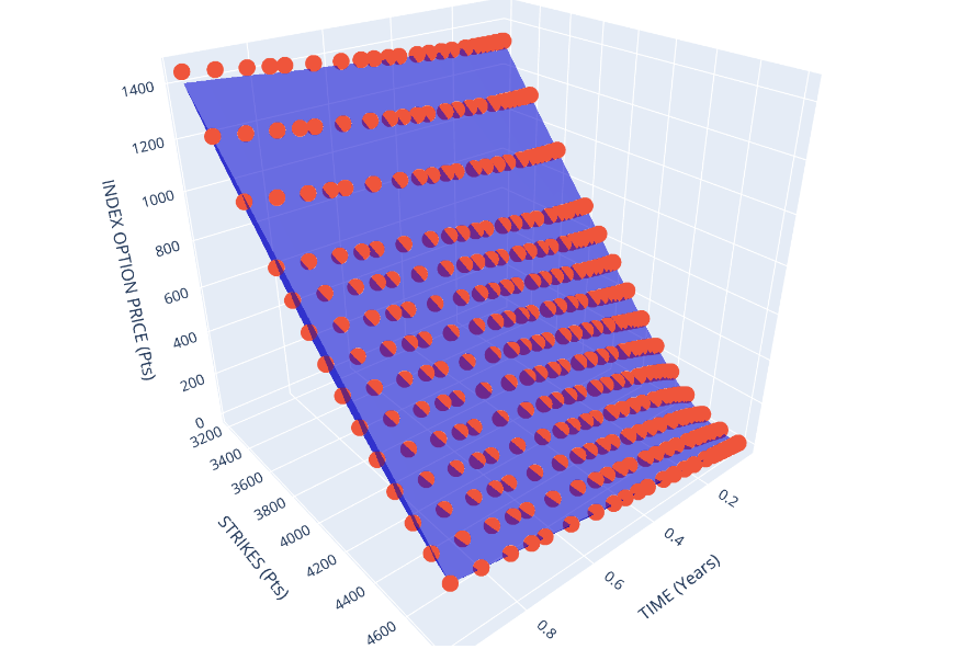
Visualise Market Prices vs Heston Prices
import plotly.graph_objects as go
from plotly.graph_objs import Surface
from plotly.offline import iplot, init_notebook_mode
init_notebook_mode()

fig = go.Figure(data=[go.Mesh3d(x=volSurfaceLong.maturity, y=volSurfaceLong.strike, z=volSurfaceLong.price, color='mediumblue', opacity=0.55)])

fig.add_scatter3d(x=volSurfaceLong.maturity, y=volSurfaceLong.strike, z=volSurfaceLong.heston_price, mode='markers')

fig.update_layout(
    title_text='Market Prices (Mesh) vs Calibrated Heston Prices (Markers)',
    scene = dict(xaxis_title='TIME (Years)',
                    yaxis_title='STRIKES (Pts)',
                    zaxis_title='INDEX OPTION PRICE (Pts)'),
    height=800,
    width=800
)

fig.show()