Beta weighting is a tool that allows us to approximate our positions in terms of the same benchmark. Today we learn how to beta weight your portfolio in python.
We will use three equivalent methods to estimate the beta coefficients of each security and then progress onto how you can beta weight your portfolio delta’s (the change in value given a unit change of the underlying) to get an approximation for how your portfolio will change with respect to a movement in your benchmark (whether it be a market index or specific security).
We will calculate beta coefficients directly using the capital asset pricing model (CAPM) definition, and through some linear algebra tools using linear regression on individual stocks and then aggregated using a closed form solution for linear regression with a specific minimisation function.
import datetime as dt
import pandas as pd
import numpy as np
from scipy import stats
from pandas_datareader import data as pdr
Specify date range for analysis
Here we begin by creating start and end dates using pythons datetime module.
start = dt.datetime(2021, 1, 1)
end = dt.datetime.now()
start, end
Select the stocks/tickers you would like to analyse
For Australian stocks, yahoo tickers require ‘.AX’ to be specified at the end of the ticker symbol. For other tickers, use the search bar in yahoo finance to work out other ticker structures. https://au.finance.yahoo.com/
stockList = ['CBA', 'NAB', 'WBC', 'ANZ','WPL']
stocks = ['^AXJO'] + [i + '.AX' for i in stockList]
stocks
Using Pandas_Datareader
Two ways of doing this:
- pdr.DataReader(stocks, ‘yahoo’, start, end)
- pdr.get_data_yahoo(stocks, start, end)
df = pdr.get_data_yahoo(stocks, start, end)
log_returns = np.log(df.Close / df.Close.shift(1)).dropna()
log_returns.head()
Option 1: Directly calculate beta
\(\frac{covariance(Market, Stock)}{variance(Market)}\)
def calc_beta(df):
    np_array = df.values
    # Market index is the first column 0
    m = np_array[:,0]
    beta = []
    for ind, col in enumerate(df):
        if ind > 0:
            # stock returns are indexed by ind
            s = np_array[:,ind]
            # Calculate covariance matrix between stock and market
            covariance = np.cov(s,m)
            beta.append( covariance[0,1]/covariance[1,1] )
    return pd.Series(beta, df.columns[1:], name='Beta')

calc_beta(log_returns)
Option 2: Use linear regression
def regression_beta(df):
    np_array = df.values
    # Market index is the first column 0
    m = np_array[:,0]
    beta = []
    for ind, col in enumerate(df):
        if ind > 0:
            s = np_array[:,ind] # stock returns are column one from numpy array
            beta.append( stats.linregress(m,s)[0] )
    return pd.Series(beta, df.columns[1:], name='Beta')

regression_beta(log_returns)
Option3: Use Matrix Algebra
For linear regression on a model of the form \(y=X\beta\), where X is a matrix with full column rank, the least squares solution,
\(\hat{\beta} = arg \min ||X\beta−y||_2 \)
\(\hat{\beta} = (X^T X)^{−1}X^Ty \)
https://stats.stackexchange.com/questions/23128/solving-for-regression-parameters-in-closed-form-vs-gradient-descent/23132#23132
def matrix_beta(df):
    # Market index is the first column 0
    X = df.values[:, [0]]
    # add an additional column for the intercept (initalise as 1's)
    X = np.concatenate([np.ones_like(X), X], axis=1)
    # Apply matrix algebra for linear regression model
    beta = np.linalg.pinv(X.T @ X) @ X.T @ df.values[:, 1:]
    return pd.Series(beta[1], df.columns[1:], name='Beta')

beta = matrix_beta(log_returns)
Define your Portfolio and make DataFrame
Calculate Beta Weighted Portfolio
units = np.array([100, 250, 300, 400, 200])
ASXprices = df.Close[-1:].values.tolist()[0]
price = np.array([round(price,2) for price in ASXprices[1:]])
value = [unit*pr for unit, pr in zip(units, price)]
weight = [round(val/sum(value),2) for val in value]
beta = round(beta,2)

Portfolio = pd.DataFrame({
    'Stock': stockList,
    'Direction': 'Long',
    'Type': 'S',
    'Stock Price': price,
    'Price': price,
    'Units': units,
    'Value': units*price,
    'Weight': weight,
    'Beta': beta,
    'Weighted Beta': weight*beta
})
Portfolio
What if we have options, let’s consider things in terms of Delta
Portfolio = Portfolio.drop(['Weight', 'Weighted Beta'], axis=1)
Portfolio['Delta'] = Portfolio['Units']
Add options to the portfolio, this is Only an example.
Options = [{'option':'CBA0Z8', 'underlying':'CBA', 'price':3.950, 'units': 2, 'delta': 0.627, 'direction': 'Short', 'type': 'Call'},
           {'option':'WPLQB9', 'underlying':'WPL', 'price':1.325, 'units': 2, 'delta': -0.425 ,'direction': 'Long', 'type': 'Put'}]

for index, row in enumerate(Options):
    Portfolio.loc[row['option']] = [row['underlying'], row['direction'], row['type'], Portfolio.loc[row['underlying']+'.AX', 'Price'],
                                    row['price'], row['units'], row['price']*row['units']*100, beta[row['underlying']+'.AX'],
                                    (row['delta']*row['units']* 100 if row['direction'] == 'Long' else -row['delta']*row['units']*100)]
Portfolio
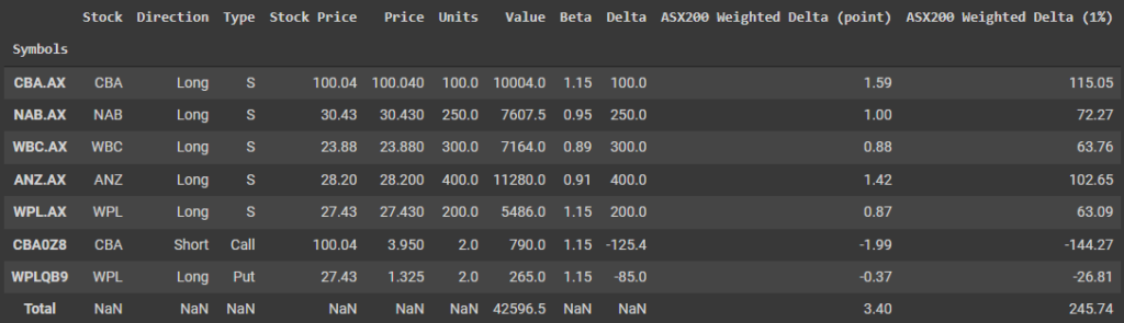
Weight the Delta’s using Beta
Portfolio['ASX200 Weighted Delta (point)'] = round(Portfolio['Beta'] * (Portfolio['Stock Price']/ASXprices[0]) * Portfolio['Delta'],2)
Portfolio['ASX200 Weighted Delta (1%)'] = round(Portfolio['Beta'] * (Portfolio['Stock Price']) * Portfolio['Delta'] * 0.01,2)
Portfolio
Total the Delta’s to get Portfolio Overview
Portfolio.loc['Total', ['Value', 'ASX200 Weighted Delta (point)', 'ASX200 Weighted Delta (1%)']] \
= Portfolio[['Value','ASX200 Weighted Delta (point)', 'ASX200 Weighted Delta (1%)']].sum()
Portfolio