In part 2 of this weather derivative series, our goal is to: complete statistical analysis on temperature data
Quick Summary – our goal:
Aim: we want to price temperature options.
Underlying: HDD/CDD index over given period.
The underlying over a temperature option is the heating/cooling degree days (HDD/CDD) index based on ‘approximation’ of average temperature and reference (/base) temperature.
\(\large T_n = \frac{T^{max}+T^{min}}{2}\)
For an individual day \(n \in N\):
- \(\large HDD_n = (T_{ref}-T_n)^+\)
- \(\large CDD_n = (T_n – T_{ref})^+\)
HDD/CDD Index for a given period \(N\):
- \(\large DD = H_n = HDD^{N} = \sum^N_n HDD_n\)
- \(\large DD = C_n = CDD^{N} = \sum^N_n CDD_n\)
Option Payoff: \(\large \xi = f(DD)\)
Example of popular OTC product: Call with Cap
\(\large \xi = min{\alpha(DD – K)^+, C}\)
where:
- payoff rates \(\large \alpha\) is commonly US\(\$2,500\) or US\(\$5,000\) [1]
- while caps \(\large C\) is commonly US\(\$500,000\) or US\(\$1,000,000\) [1]
References:
[1] Statistical Analysis of Financial Data in R (Rene Carmona, 2014)
Dataset
Weather Observations for Sydney, Australia – Observatory Hill:

Dataset Start to End:
- Weather Station 1: 1-Jan 1859 – 30-Aug 2020
- Weather Station 2: 18-Oct 2017 – 3-Jul 2022
Data available:
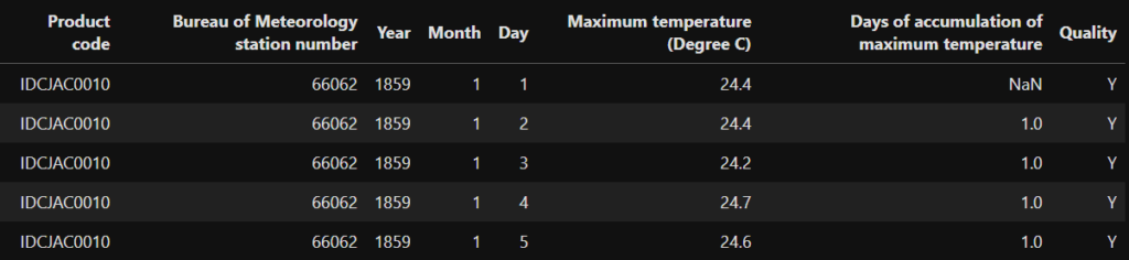
- Maximum Temperature
- Minimum Temperature
import numpy as np
import pandas as pd
import datetime as dt
import matplotlib.pyplot as plt

max_temp = pd.read_csv('https://raw.githubusercontent.com/ASXPortfolio/jupyter-notebooks-data/main/maximum_temperature.csv')
min_temp = pd.read_csv('https://raw.githubusercontent.com/ASXPortfolio/jupyter-notebooks-data/main/minimum_temperature.csv')

max_temp.head()
Now we check for missing data. Are these the same days? If not will have to drop all rows (days) with at least value missing.
max_temp.isnull().value_counts(),min_temp.isna().value_counts()

count = 0
for mx, mn in zip(np.where(max_temp.isnull())[0], np.where(min_temp.isnull())[0]):
    if mx != mn:
        count += 1

print('Number of Misaligned Null Values: ', count)
Create cleaned max min temperature dataframe
def datetime(row):
return dt.datetime(row.Year,row.Month,row.Day)
max_temp['Date'] = max_temp.apply(datetime,axis=1)
min_temp['Date'] = min_temp.apply(datetime,axis=1)
max_temp.set_index('Date', inplace=True)
min_temp.set_index('Date', inplace=True)
drop_cols = [0,1,2,3,4,6,7]
max_temp.drop(max_temp.columns[drop_cols],axis=1,inplace=True)
min_temp.drop(min_temp.columns[drop_cols],axis=1,inplace=True)
max_temp.rename(columns={'Maximum temperature (Degree C)':'Tmax'}, inplace=True)
min_temp.rename(columns={'Minimum temperature (Degree C)':'Tmin'}, inplace=True)
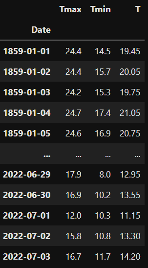
temps = max_temp.merge(min_temp,how='inner',left_on=['Date'],right_on=['Date'])
def avg_temp(row):
return (row.Tmax+row.Tmin)/2
temps['T'] = temps.apply(avg_temp,axis=1)
# drop na values here
temps = temps.dropna()
temps
May may also want to use the pandas .describe() function to check some basic statistics on each column.
Indicate winter and summer periods
Here in Australia:
- Winter ~ May-Oct
- Summer ~ Nov-Apr
temps_season = temps.copy(deep=True)
temps_season['month'] = temps_season.index.month
mask = (temps_season['month'] >= 5) & (temps_season['month'] <= 10)
temps_season['winter'] = np.where(mask,1,0)
temps_season['summer'] = np.where(temps_season['winter'] != 1,1,0)
temps_season
Data Visualisation
# timeseries plot - all data
temps[:].plot(figsize=(8,6))
plt.show()

# timeseries plot - ~14 years
temps[-5000:].plot(figsize=(8,6))
plt.show()

#temperature distributions in histogram
plt.figure(figsize=(8,6))
temps.Tmax.hist(bins=60, alpha=0.6, label='Tmax')
temps.Tmin.hist(bins=60, alpha=0.6, label='Tmin')
temps['T'].hist(bins=60, alpha=0.8, label='T')
plt.legend()
plt.show()
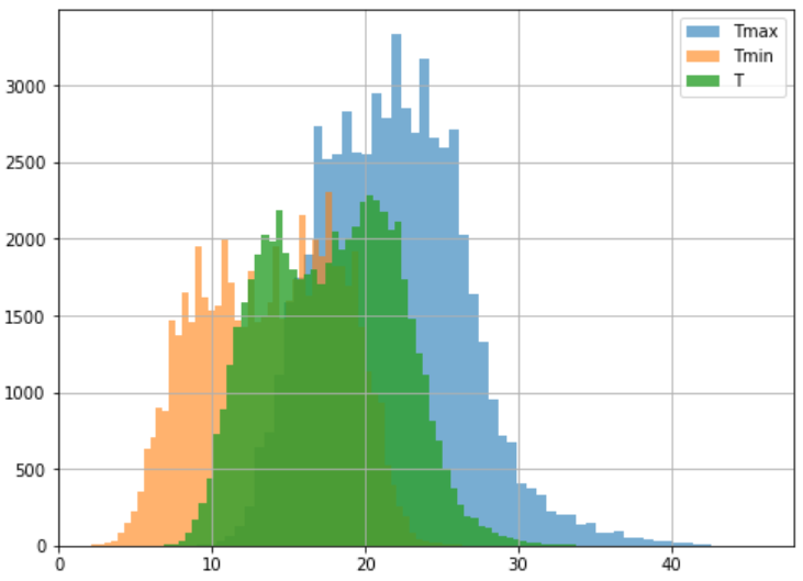
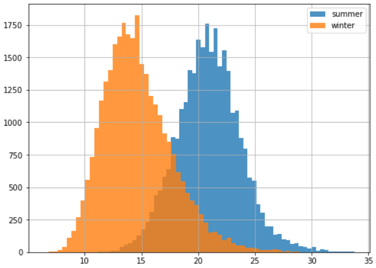
Bimodal Distribution
The two peaks reflect both the summer and winter months.
plt.figure(figsize=(8,6))
temps_season[temps_season['summer'] == 1]['T'].hist(bins=60, alpha=0.8, label='summer')
temps_season[temps_season['winter'] == 1]['T'].hist(bins=60, alpha=0.8, label='winter')
plt.legend()
plt.show()
Temperature Records
Compile list of min and max records for each month in data timeframe.
date_list = temps.index.tolist()
mth_temps = pd.DataFrame(data=date_list, index=date_list).resample('MS')[0].agg([min, max])
mth_temps['month'] = mth_temps.index.month
def min_max_temps(row):
    stats = temps[(temps.index >= row['min']) & (temps.index <= row['max'])].agg([min, max])
    row['Tmax_max'] = stats.loc['max', 'Tmax']
    row['Tmax_min'] = stats.loc['min', 'Tmax']
    row['Tmin_max'] = stats.loc['max', 'Tmin']
    row['Tmin_min'] = stats.loc['min', 'Tmin']
    row['T_max'] = stats.loc['max', 'T']
    row['T_min'] = stats.loc['min', 'T']
    return row

mth_temps = mth_temps.apply(min_max_temps,axis=1)
mth_temps
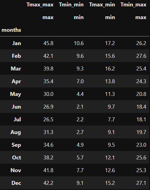
Let’s look at the Temperature Extreme’s on record
Now we can group on whichever seasons we would like, so here we aggregate on months from 1857-2022 to get the:
- maximum Tmax’s
- minimum Tmin’s
Also interesting to inspect
- maximum Tmin’s
- minimum Tmax’s
grouped_mths = mth_temps.groupby(mth_temps.month)[['Tmax_max', 'Tmax_min', 'Tmin_max', 'Tmin_min','T_max','T_min']].agg([min, max])
grouped_mths['months'] = ['Jan','Feb','Mar','Apr','May','Jun','Jul','Aug','Sep','Oct','Nov','Dec']
grouped_mths = grouped_mths.set_index('months')
grouped_mths[[('Tmax_max', 'max'),('Tmin_min', 'min'),('Tmax_min', 'min'),('Tmin_max', 'max')]]
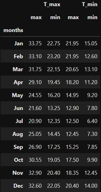
Let’s look at our Temperature Options Underlying: “Avg Temp”
This time we will look at the max and min’s for both T_max and T_min for each month on record. Again we aggregate on months from 1857-2022 to get the:
- maximum T_max’s
- minimum T_min’s
Also interesting to inspect
- maximum T_min’s
- minimum T_max’s
grouped_mths[[('T_max', 'max'),('T_max', 'min'),('T_min', 'max'),('T_min', 'min')]]