
In part 3 of this weather derivative series, our goal is to de-trend and remove seasonality using statsmodels decompose function classical decomposition using moving averages.
Quick Summary – our goal:
Aim: we want to price temperature options.
Underlying: HDD/CDD index over given period.
The underlying over a temperature option is the heating/cooling degree days (HDD/CDD) index based on ‘approximation’ of average temperature and reference (/base) temperature.
\(\large T_n = \frac{T^{max}+T^{min}}{2}\)
For an individual day \(n \in \):
- \(\large HDD_n = (T_{ref}-T_n)^+\)
- \(\large CDD_n = (T_n – T_{ref})^+\)
HDD/CDD Index for a given period \(N\):
- \(\large DD = H_n = HDD^{N} = \sum^N_n HDD_n\)
- \(\large DD = C_n = CDD^{N} = \sum^N_n CDD_n\)
Option Payoff: \(\large \xi = f(DD)\)
Example of popular OTC product: Call with Cap
\(\large \xi = min{\alpha(DD – K)^+, C}\)
where:
- payoff rates \(\large \alpha\) is commonly US\(\$2,500\) or US\(\$5,000\) [1]
- while caps \(\large C\) is commonly US\(\$500,000\) or US\(\$1,000,000\) [1]
References:
[1] Statistical Analysis of Financial Data in R (Rene Carmona, 2014)
Decompose Time-Series Components
Time series decomposition is a technique that splits a time series into several components, each representing an underlying pattern category, trend, seasonality, and noise.
- Trend: decreasing, constant, or increasing over time?
- Seasonality: what is the periodic signal?
- Noise: variability in the data that cannot be explained by the model
statsmodels: seasonal_decompose
This is a naive decomposition – classical decomposition. More sophisticated methods should be preferred.
The additive model is \(y_t = T_t + S_t + e_t\)
The results are obtained by first estimating the trend by applying a convolution filter to the data. The trend is then removed from the series and the average of this de-trended series for each period is the returned seasonal component. The steps in classical decomposition are as follows:
1) compute the trend-cycle component \(\hat{T_t}\) using an m-MA (moving average)
2) calculate de-trended series \(y_t – \hat{T_t}\)
3) estimate seasonal component \(\hat{S_t}\), by averaging the detrended values for that season (in our case, this is each day of the year). Seasonal component values are adjusted to ensure they add to zero.
4) the remainder is calculated \(e_t = y_t – \hat{T_t} – \hat{S_t}\)
import numpy as np
import pandas as pd
import datetime as dt
import matplotlib.pyplot as plt

from statsmodels.graphics.api import qqplot
from statsmodels.tsa.stattools import adfuller
from statsmodels.tsa.seasonal import seasonal_decompose
from statsmodels.graphics.tsaplots import plot_acf, plot_pacf
from statsmodels.tsa.ar_model import AutoReg, ar_select_order, AutoRegResults
Please use the temperature data as contructed in the previous part of this [series](https://quantpy.com.au/weather-derivatives/statistical-analysis-of-temperature-data/).
When you execute the following code, we can clearly see an upward trend in temperature over time, and varying volatility.
temps.sort_index(inplace=True)
temps['T'].rolling(window = 365*10).mean().plot(figsize=(8,4), color="tab:red", title="Rolling mean over annual periods")
temps['T'].rolling(window = 365*10).var().plot(figsize=(8,4), color="tab:red", title="Rolling variance over annual periods");
Use seasonal_decompose function
decompose_result = seasonal_decompose(temps['T'], model='additive', period=int(365), extrapolate_trend='freq')
trend = decompose_result.trend
seasonal = decompose_result.seasonal
residual = decompose_result.resid
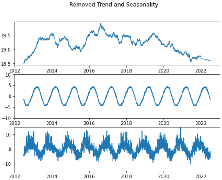
### Visualise All Data
decompose_result.plot()
plt.show()
### Visualise 10 years
years_examine = 365*10
fig, axs = plt.subplots(3, figsize=(8,6))
fig.suptitle('Removed Trend and Seasonality')
axs[0].plot(trend[-years_examine:])
axs[1].plot(seasonal[-years_examine:])
axs[1].set_ylim([-10,10])
axs[2].plot(residual[-years_examine:])
axs[2].set_ylim([-15,15])
Testing for Stationarity with Dicky-Fuller
We can perform Dicky-Fuller test functionality available with the statsmodels library. Below we’ll test the stationarity of our time-series with this functionality and try to interpret its results to better understand it.
Unit Root Test, null hypothesis is that unit root exists.
dftest = adfuller(residual, autolag = 'AIC')

print("1. ADF : ",dftest[0])
print("2. P-Value : ", dftest[1])
print("3. Num Of Lags : ", dftest[2])
print("4. Num Of Observations Used For ADF Regression and Critical Values Calculation :", dftest[3])
print("5. Critical Values :")
for key, val in dftest[4].items():
    print("\t",key, ": ", val)
Check residual distribution
residual.hist(bins=60, figsize=(8,6))
Analysis of Serial Correlations
Below we are also plotting auto-correlation plot for time-series data as well. This plot helps us understand whether present values of time-series are positively correlated, negatively correlated or not related at all with past values.
statsmodels library provides ready to use method plot_acf as a part of module statsmodels.graphics.tsaplots
plot_acf(residual, lags=100)
plt.show()
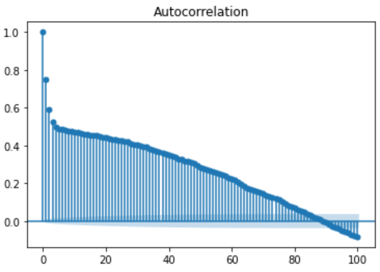
Above we can see significant serial correlation. Since the auto-correlation funtion does not seem to vanish after after a finite number of lags, we do not try and fit a moving average model.
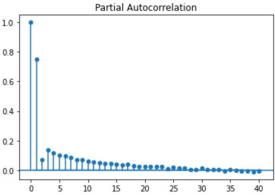
Determine AR order by use of PACF & AIC Criterion
PACF is a partial auto-correlation function. Basically instead of finding correlations of present values with lags like ACF, it finds correlation of the residuals.
These residuals remain after removing the effects which are already explained by the earlier lag(s) with the next lag value. i.e. We remove already found variations before we find the next correlation.
plot_pacf(residual, lags=40)
plt.show()
Akaike Information Criterion (AIC)
AIC is a single number score that can be used to determine which of multiple models is most likely to be the best model for a given dataset. AIC works by evaluating the model’s fit on the training data, and adding a penalty term for the complexity of the model.
\(\large AIC = -2ln(L) + 2k\)
AIC equation, where L = likelihood and k = # of parameters. AIC uses a model’s maximum likelihood estimation (log-likelihood) as a measure of fit. Log-likelihood is a measure of how likely one is to see their observed data, given a model. The model with the maximum likelihood is the one that “fits” the data the best.
The desired result is to find the lowest possible AIC, which indicates the best balance of model fit with generalizability. This serves the eventual goal of maximizing fit on out-of-sample data.
residuals = residual.copy(deep=True)
residuals.index = pd.DatetimeIndex(residuals.index).to_period('D')

mod = ar_select_order(residuals, maxlag=40, ic='aic', old_names=True)

aic = []
for key, val in mod.aic.items():
    if key != 0:
        aic.append((key[-1], val))

aic.sort()
x,y = [x for x,y in aic],[y for x,y in aic]

plt.scatter(x, y)
plt.plot([0,40],[y[15],y[15]], 'tab:orange')
plt.text(3,y[15]+0.002, '{0}'.format(round(y[15],3)),color='tab:orange')
plt.plot([0,40],[y[20],y[20]], 'k--')
plt.text(3,y[20]-0.004, '{0}'.format(round(y[20],3)))
plt.title("AIC Criterion")
plt.xlabel("Lags in AR Model")
plt.ylabel("AIC")
plt.show()
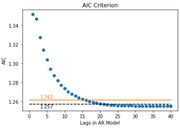
Fitting a AR with lags=15
Interpreting the results with statsmodels .summary()
model = AutoReg(residuals, lags=15, old_names=True,trend='n')
model_fit  = model.fit()
coef = model_fit.params
res = model_fit.resid
res.index = res.index.to_timestamp()
print(model_fit.summary())

fig, axs = plt.subplots(2,2, figsize=(8,6))
fig.suptitle('Residuals after AR(15) model')
axs[0,0].plot(res)
axs[1,0].plot(res[-200:])
plot_acf(res, lags=20, ax=axs[0,1])
plot_pacf(res, lags=20, ax=axs[1,1])
plt.show()

from scipy.stats import norm
qqplot(res, marker='x', dist=norm, loc=0, scale=np.std(res), line='45')
plt.show()
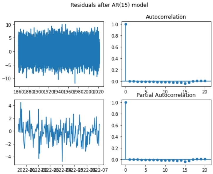
The auto-correlation function of the raw residuals of the AR(15) model fitted to the remainder component of the daily temperature in Sydney, looks like white noise now!
The serial correlation in the data appears to have been captured by the AR(15) model. We have our model, including the trend, seasonality and AR(15) model.